STAT 3360 Notes
Table of Contents
1 Continuous Probability Distribution
1.1 Probability Density Function
1.1.1 Definition
- The function \(f(x)\) which describes the probability distribution of a continuous random variable \(X\) is called a Probability Density Function.
- The input (the \(x\) inside \(f(\cdot)\)) of \(f(x)\) is a value of the continuous random variable \(X\).
- The output (function value) of \(f(x)\) is NOT the probability of the event \(X=x\).
- This is different from the discrete case, and is the reason why we study discrete distribution and continuous distribution separately.
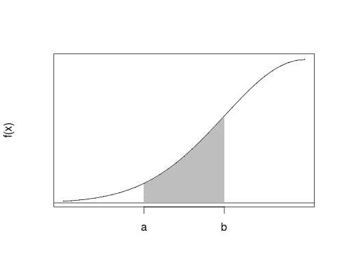
The probability density function is defined in such a way that the probabilities of the events "\(X \in (a, b)\)", "\(X \in [a, b)\)", "\(X \in (a, b]\)", and "\(X \in [a, b]\)" are all equal to \(\int_a^b f(x) dx\). That is, \[ \boxed{ P(X \in (a, b)) = P(a < X < b) = \int_{a}^{b} f(x) dx } \] \[ \boxed{ P(X \in [a, b)) = P(a \le X < b) = \int_{a}^{b} f(x) dx } \] \[ \boxed{ P(X \in (a, b]) = P(a < X \le b) = \int_{a}^{b} f(x) dx } \] \[ \boxed{ P(X \in [a, b]) = P(a \le X \le b) = \int_{a}^{b} f(x) dx } \]
We know the definite integral \(\int_a^b f(x) dx\) represents the area under the curve of \(f(x)\) between \(a\) and \(b\).
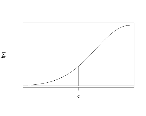
We see that the endpoint, as a single point, does not contribute to the probability of the whole interval. The reason is, for any single point \(c\), \[ \boxed{ P(X = c) } = P(X \in [c, c]) = \int_c^c f(x) dx = \boxed{0} \] Note: the probability of the event "\(X = x\)" is \(0\), NOT \(f(x)\), which is different from the discrete case.
Geometrically, at a single point, the "area" under the curve of \(f(x)\) is \(0\).
- To summarize, for continuous random variables,
- we don't care about probabilities like \(P(X=x)\), which is always \(0\)
- we care about the probabilities like \(P(X \in (a, b))\), \(P(X \in [a, b))\), \(P(X \in (a, b])\), and \(P(X \in [a, b])\), which are all equal to \(\int_a^b f(x) dx\)
1.1.2 Requirements
- Not all functions can work as probability density functions. An eligible probability density function must satisfy
- \(f(x) \ge 0\) for all \(x \in (-\infty, \infty)\)
- This ensures the probability \(P(x \in (a, b)) = \int_a^b f(x) dx\) is always non-negative.
- \(\int_{-\infty}^{\infty} f(x) dx = 1\)
- This ensures \(P(x \in (-\infty, \infty)) = 1\)
- \(f(x) \ge 0\) for all \(x \in (-\infty, \infty)\)
1.1.3 Example
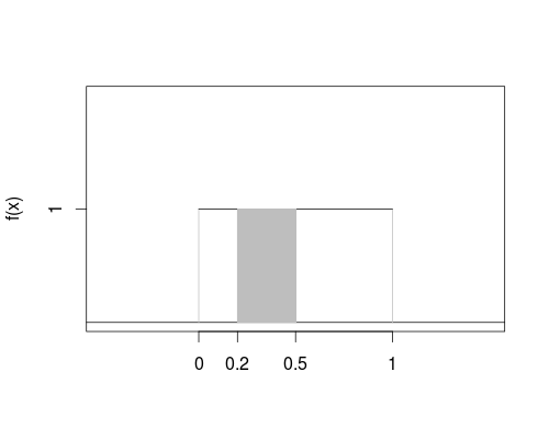
- Suppose \[f(x) = \left\{ \begin{array}{ll} 1, & \text{ if } x \in [0, 1] \\ 0, & \text{ otherwise } \end{array} \right.\]
- Then
- \(f(x)\) is an eligible probability density function because
- \(f(x) \ge 0\) for all \(x\)
\(\int_{-\infty}^{\infty} f(x) dx\)
\(= \int_{-\infty}^{0} f(x) dx + \int_{0}^{1} f(x) dx + \int_{1}^{\infty} f(x) dx\)
\(= \int_{-\infty}^{0} 0 dx + \int_{0}^{1} 1 dx + \int_{1}^{\infty} 0 dx\)
\(= 0 \big|_{-\infty}^{0} + x \big|_{0}^{1} + 0 \big|_{1}^{\infty}\)
\(= 0 + 1 + 0 = 1\)
\(P(X \in (0.2, 0.5]) = \int_{0.2}^{0.5} 1 dx = x \big|_{0.2}^{0.5} = 0.5 - 0.2 = 0.3\)
- \(f(x)\) is an eligible probability density function because
1.2 Cumulative Probability
1.2.1 Introduction
- For discrete distributions, we have already seen that using cumulative probability \(P(X \le k)\), we can calculate the probabilities of all other events.
- For continuous distributions, this is also true.
1.2.2 Definition
- For a random variable \(X\) and a constant \(c\), the probability \(P(X \le c)\) is called the Cumulative Probability of \(X\) at \(c\).
1.2.3 Application
- Suppose \(X\) is a continuous random variable and \(a < b\) and \(c\) are all constants.
- Given the cumulative probability \(P(X \le c) = \int_{-\infty}^{c} f(x) dx\), we can calculate \(P(X < c)\), \(P(X \ge c)\) and \(P(X > c)\) in the following way:
- \(\boxed{P(X < c)} = \int_{-\infty}^{c} f(x) dx = \boxed{P(X \le c)}\)
- \(\boxed{P(X \ge c)} = 1 - P(X < c) = \boxed{1 - P(X \le c)}\)
- \(\boxed{P(X > c)} = \boxed{1 - P(X \le c)}\)
- Given the cumulative probabilities \(P(X \le a) = \int_{-\infty}^{a} f(x) dx\) and \(P(X \le b) = \int_{-\infty}^{b} f(x) dx\), we can calculate \(P(a \le X < b)\), \(P(a < X \le b)\) and \(P(a \le X \le b)\) in the following way:
- \(\boxed{P(a < X < b)} = P(X < b) - P(X \le a) = \boxed{P(X \le b) - P(X \le a)}\)
- \(\boxed{P(a \le X < b)} = P(X < b) - P(X < a) = \boxed{P(X \le b) - P(X \le a)}\)
- \(\boxed{P(a < X \le b)} = \boxed{P(X \le b) - P(X \le a)}\)
- \(\boxed{P(a \le X \le b)} = P(X \le b) - P(X < a) = \boxed{P(X \le b) - P(X \le a)}\)
1.2.4 Lower and Upper Percentile
- For a continuous random variable \(X\),
- \(q\) is called the lower \(p\) percentile of the distribution of \(X\) if \(\boxed{ P(X \le q) = p\% }\). That is, the probability that \(X\) is less than or equal to \(q\) is \(p\%\).
- \(q\) is called the upper \(p\) percentile of the distribution of \(X\) if \(\boxed{ P(X > q) = p\% }\). That is, the probability that \(X\) is greater than \(q\) is \(p\%\).
- the lower \(p\) percentile is just the upper \((100 - p)\) percentile.
- the upper \(p\) percentile is just the lower \((100 - p)\) percentile.
- Example
- In the following plot, \(P(X \le -1) = 16\%\), so
- \(q = -1\) is the lower \(16\) percentile,
- \(q = -1\) is the upper \((100 - 16) = 84\) percentile.
In the following plot, \(P(X > 0.5) = 31\%\), so
- \(q = 0.5\) is the upper \(31\) percentile,
- \(q = 0.5\) is the lower \((100 - 31) = 69\) percentile
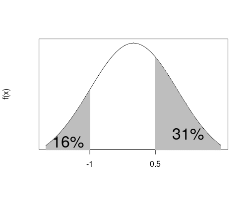
- In the following plot, \(P(X \le -1) = 16\%\), so
1.2.5 Cumulative Probability and Percentile
- We note that cumulative probability and lower percentile are inverse to each other:
- cumulative probability: given \(q\), find \(p = P(X \le q)\).
- lower percentile: given \(p = P(X \le q)\), find the unknown \(q\).
2 Normal Distribution
2.1 Introduction
- For discrete distributions, we have studied two special cases: Binomial distribution and Poisson distribution.
- For continuous distributions, we will now study an important special case: Normal distribution.
2.2 Normal Random Variable
- Suppose \(\mu\) and \(\sigma > 0\) are constants and \(X\) is a continuous random variable whose values are all real numbers.
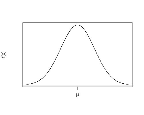
\(X\) is called a Normal random variable if its probability mass distribution is \[ \boxed{ f(x) = \frac{1}{\sqrt{2\pi\sigma^2}} \cdot e^{-\frac{(x - \mu)^2}{2\sigma^2}}, -\infty < x < \infty} \]
Note: this Normal probability density function is so complicated that we never directly use it in this course.
2.3 Normal Distribution
2.3.1 Definition
- The probability distribution of the above Normal random variable \(X\) is called Normal Distribution with parameters \(\mu\) and \(\sigma^2\), which is denoted by \(\boxed{ X \sim N(\mu, \sigma^2) }\).
2.3.2 Properties
- If \(X\sim N(\mu, \sigma^2)\), then
- the expected value of \(X\) is \[ \boxed{ E(X) = \mu } \]
- the variance of \(X\) is \[ \boxed{ Var(X) = \sigma^2 } \]
- the standard deviation of \(X\) is \[ \boxed{ SD(X) = \sigma } \]
2.4 Standard Normal Distribution
2.4.1 Definition
- If \(X \sim N(\mu = 0, \sigma^2 = 1)\), then the distribution of \(X\) is called Standard Normal Distribution.
- By convention, we use \(Z\) to represent the standard Normal distribution.
2.4.2 Cumulative Probability
- For standard Normal \(Z\), the cumulative probability at point \(z\) is just \(P(Z \le z)\).
- As discussed before, once the cumulative probabilities \(P(Z \le z)\) are known, we can calculate all the other probabilities.
- As for Binomial and Poisson distributions, the cumulative probability of standard Normal distribution is so hard to calculate that tables are made for people to directly find \(P(Z \le z)\) for various values of \(z\).
2.4.3 Cumulative Probability Table
- Usage 1: Finding Cumulative Probability
- Quite similar to the Binomial and Poisson distributions, we can directly find the cumulative probability of standard Normal distribution from the table.
- However, there is a difference in the organization between the standard Normal table and Binomial/Poisson table.
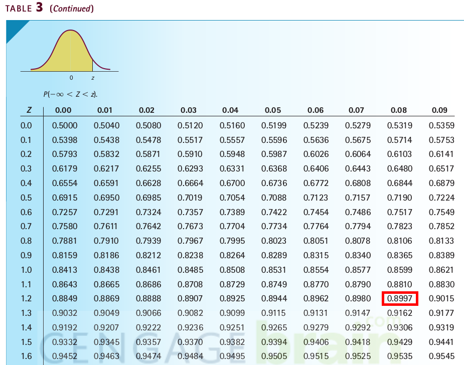
- Each row in the table represents the integer and the first decimal place of the number \(z\)
- Each column in the table represents the second decimal place of the number \(z\)
- Each intersection cell represents the cumulative probability \(P(Z \le z)\) for standard Normal \(Z\)
Example
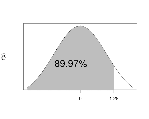
- What is the cumulative probability \(P(Z \le 1.28)\) for the standard Normal random variable \(Z\)?
- \(1.28\) can be split into \(1.2\) and \(0.08\), so we
- find the row for \(1.2\)
- find the column for \(0.08\)
- Then the intersection cell in the table tells us \(P(Z \le 1.28) = 0.8897 = 89.97\%\)
- Usage 2: Finding Lower Percentile
- We already know that cumulative probability and lower quantile are inverse to each other, so from the cumulative probability table we can also find the lower \(p\) percentile for a given \(p\).
- Since upper \(p\) percentile = lower \((100-p)\) percentile, we can also get the upper \(p\) percentile by finding the lower \((100-p)\) percentile.
Example 1
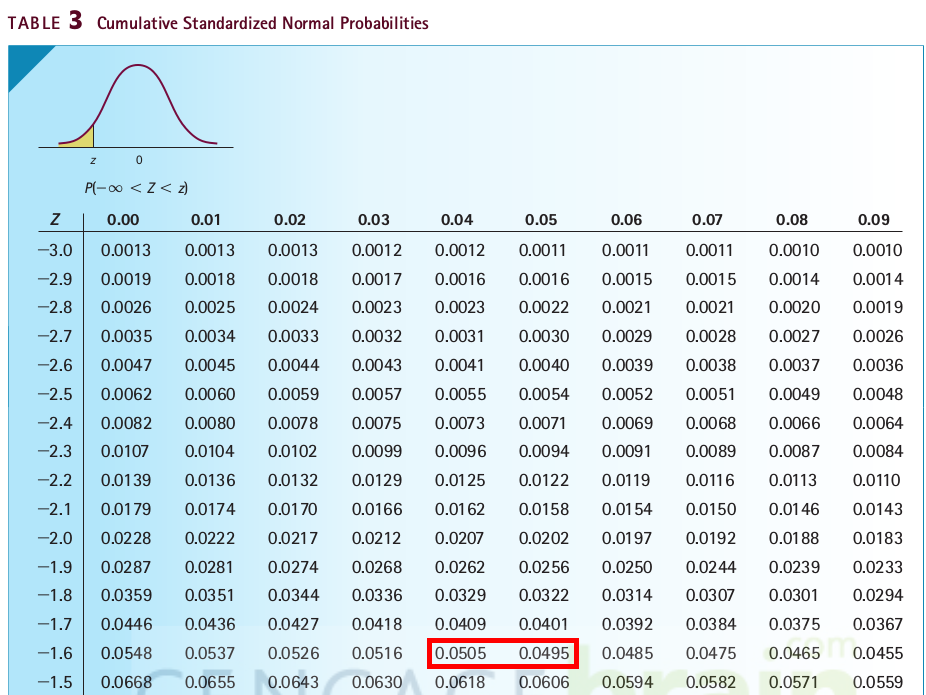
- What is the lower \(5\) percentile for the standard Normal distribution?
- By definition, we need find \(q\) such that \(P(Z \le q) = 5\% = 0.05\). That is, we need find from the table the cell giving \(0.05\).
- In the table, there is no cell exactly equal to \(0.05\), but \(P(Z \le -1.65) = 0.0495\) and \(P(Z \le -1.64) = 0.0505\), so we may use \(q = -1.65\) or \(q = -1.64\) as the lower \(5\) percentile.
Example 2
- What is the upper \(10\) percentile for the standard Normal distribution?
- From the cumulative probability table, we can only find lower percentiles.
- Therefore, to find an upper percentile, we should first convert it into the corresponding lower percentile.
- By the relationship between upper quantile and lower quantile, we have upper \(10\) percentile = lower \((100 - 10) = 90\) percentile, so we should find the lower \(90\) percentile from the table.
- In the table, there is no cell exactly equal to \(0.90\), but \(P(Z \le 1.28) = 0.8997\), so we may use \(q = 1.28\) as the lower \(90\) percentile, which is also upper \(10\) percentile.
2.5 Standardization of Normal Random Variable
2.5.1 Introduction
- For the standard Normal distribution, we have a cumulative probability table and can conveniently find the cumulative probability or lower percentile of interest.
- What if we have a non-standard Normal distribution? How do we get its cumulative probability? How do we find its lower and upper percentile?
- The answer is, there is a bridge between non-standard and standard Normal distributions so that we can convert the results about standard Normal into those about non-standard Normal distributions. The bridge is just the standardization given by the following theorem.
2.5.2 Thoerem
- If \(X \sim N(\mu, \sigma^2)\), then \[ \boxed{Z = \frac{X - \mu}{\sigma} \sim N(0, 1)} \]
2.5.3 Formulas Based on the Theorem
- Therefore, if \(X \sim N(\mu, \sigma^2)\), then \[ \boxed{P(X \le c)} = P(X - \mu \le c - \mu) = P \left( \frac{X - \mu}{\sigma} \le \frac{c - \mu}{\sigma} \right) = \boxed{ P \left( Z \le \frac{c - \mu}{\sigma} \right) } \]
Suppose \(q_x\) is the lower \(p\) percentile of \(X\) and \(q_z\) is the lower \(p\) percentile of \(Z\). Then
- by definition, \(p = P(X \le q_x) = P(Z \le q_z)\)
- by the formula, \(P(X \le q_x) = P(Z \le \frac{q_x - \mu}{\sigma})\)
- combining the previous two lines, we have \(P(Z \le q_z) = P(Z \le \frac{q_x - \mu}{\sigma})\) and thus \(q_z = \frac{q_x - \mu}{\sigma}\)
- if \(q_z\) if known, then we can get the value of \(q_x\) by
\[ \boxed{q_x = q_z \sigma + \mu} \]
- Similarly, when \(q_x\) is the upper \(p\) percentile of \(X\) and \(q_z\) is the upper \(p\) percentile of \(Z\), we still have \[ \boxed{q_x = q_z \sigma + \mu} \]
2.5.4 Example
- If \(X \sim N(10, 4)\), then
- \(\mu = 10\), \(\sigma^2 = 4\) and thus \(\sigma = 2\)
- by formula \(Z = \frac{X - 10}{2} \sim N(0, 1)\)
- what is the probability \(P(X \le 8)\)?
- \(P(X \le 8) = P(Z \le \frac{8 - 10}{2}) = P(Z \le -1)\). From the cumulative probability table of standard Normal distribution, we get \(P(Z \le -1) = 0.1587 = 15.87\%\).
- what is the probability \(P(X > 7)\)?
- \(P(X > 7) = 1 - P(X \le 7) = 1 - P(Z \le \frac{7 - 10}{2}) = P(Z \le -1.5)\). From the cumulative probability table of standard Normal distribution, we get \(P(Z \le -1.5) = 0.0668 = 6.68\%\).
- What is the probability \(P(7 < X < 8)\)?
- \(P(7 < X < 8) = P(X \le 8) - P(X \le 7) = 15.87\% - 6.68\% = 9.19\%\).
- What is the lower \(10\) percentile of \(X\)?
- first, from the cumulative probability table for standard Normal distribution, we know the lower \(10\) percentile for standard Normal \(Z\) is \(q_z = -1.28\)
- second, using the formula \(q_x = q_z \sigma + \mu\), we know the lower \(10\) percentile of \(X\) is \(q_x = -1.28 \cdot 2 + 10 = 7.44\).
- What is the upper \(10\) percentile of \(X\)?
- first, from the cumulative probability table for standard Normal distribution, we know the upper \(10\) percentile for standard Normal \(Z\) is \(q_z = 1.28\)
- second, using the formula \(q_x = q_z \sigma + \mu\), we know the upper \(10\) percentile of \(X\) is \(q_x = 1.28 \cdot 2 + 10 = 12.56\).
2.6 Word Problem
2.6.1 Example
- Suppose the students' scores (decimal values) follow a Normal distribution with mean \(80\) and variance \(9\).
- Q1: What is the probability that a student's score is above \(82\)?
- First, write down the information in mathematical language.
- Let \(X\) be the score of a student, then we know \(X \sim N(\mu = 80, \sigma^2 = 9)\) and thus the standard deviation \(\sigma = \sqrt{\sigma^2} = \sqrt{9} = 3\)
- We are asked about \(P(X > 82)\)
- By the formula \(P(X \le c) = P(Z \le \frac{c - \mu}{\sigma})\), we have \(P(X > 82) = 1 - p(X \le 82) = 1 - P(Z \le \frac{82 - 80}{3}) = 1 - P(Z \le 0.67)\).
- From the cumulative probability table for standard Normal, we have \(P(Z \le 0.67) = 0.7486\), so \(P(X > 82) = 1 - P(Z \le 0.67) = 1 - 0.7486 = 0.2514\), ie, \(P(X > 82) = 25.14\%\).
- First, write down the information in mathematical language.
- Q2: What is the lower \(10\) percentile of \(X\)?
- first, from the cumulative probability table for standard Normal distribution, we know the lower \(10\) percentile for standard Normal \(Z\) is \(q_z = -1.28\)
- second, using the formula \(q_x = q_z \sigma + \mu\), we know the lower \(10\) percentile of \(X\) is \(q_x = -1.28 \cdot 3 + 80 = 76.16\).
3 Sampling Distribution of Sample Mean
3.1 Theorem
- Suppose
- the random variable \(X \sim N(\mu, \sigma^2)\),
- \(X_1, X_2, \dots, X_n\) are \(n\) observations of \(X\),
- \(\bar{X} = \frac{\sum\limits_{i=1}^{n} X_i}{n}\) is the sample mean of \(X_1, X_2, \dots, X_n\).
- Then \[ \boxed{ \bar{X} \sim N \left( \mu, \frac{\sigma^2}{n} \right) } \]
3.2 Formulas Based on the Theorem
- From the Theorem, we get
- \(\boxed{ \mu_{\bar{x}} = E(\bar{X}) = \mu }\)
- \(\boxed{ \sigma_{\bar{x}}^2 = Var(\bar{X}) = \frac{\sigma^2}{n} }\)
- \(\boxed{ \sigma_{\bar{x}} = SD(\bar{X}) } = \sqrt{Var(\bar{X})} = \sqrt{\frac{\sigma^2}{n}} = \boxed{ \frac{\sigma}{\sqrt{n}} }\)
- Using the results in "Normal Distribution", we get
- \(\boxed{ P(\bar{X} \le c)} = P \left( Z \le \frac{c - \mu_{\bar{x}}}{\sigma_{\bar{x}}} \right) = P \left( Z \le \frac{c - \mu}{\sigma/\sqrt{n}} \right) = \boxed{ P \left( Z \le \frac{\sqrt{n} (c - \mu)}{\sigma} \right) }\) where \(Z\) is a standard Normal random variable.
- if \(q_{\bar{x}}\) is the lower \(p\) percentile of \(\bar{X}\) and \(q_z\) is the lower \(p\) percentile of standard Normal \(Z\), then \[ \boxed{ q_{\bar{x}} } = q_z \sigma_{\bar{x}} + \mu_{\bar{x}} = \boxed{ q_z \cdot \frac{\sigma}{\sqrt{n}} + \mu } \]
- if \(q_{\bar{x}}\) is the upper \(p\) percentile of \(\bar{X}\) and \(q_z\) is the upper \(p\) percentile of standard Normal \(Z\), then \[ \boxed{ q_{\bar{x}} } = q_z \sigma_{\bar{x}} + \mu_{\bar{x}} = \boxed{ q_z \cdot \frac{\sigma}{\sqrt{n}} + \mu } \]
3.3 Example
- Suppose the students' scores (decimal values) follows a Normal distribution with mean \(80\) and variance \(9\).
- Q1: If we randomly select \(9\) students, what is the probability that their average score is above \(82\)?
- First, write down the information in mathematical language.
- Let \(X\) be the score of a student, then we know \(X \sim N(\mu = 80, \sigma^2 = 9)\) and thus the standard deviation \(\sigma = \sqrt{9} = 3\)
- There are \(9\) observations of \(X\), so \(n = 9\) and \(\bar{X}\) is the average of the \(9\) observations
- We are asked about \(P(\bar{X} > 82)\), which equals \(1 - P(\bar{X} \le 82)\)
- By the formula \(P(\bar{X} \le c) = P \left( Z \le \frac{\sqrt{n} (c - \mu)}{\sigma} \right)\), we have \(P(\bar{X} \le 82) = P \left( Z \le \frac{\sqrt{9} (82 - 80)}{3} \right) = P(Z \le 2)\)
- From the cumulative probability table for standard Normal, we have \(P(Z \le 2) = 0.9772\), so \(P(\bar{X} > 82) = 1 - P(\bar{X} \le 82) = 1 - P(Z \le 2) = 1 - 0.9772 = 0.0228\), ie, \(P(\bar{X} > 82) = 2.28\%\).
- First, write down the information in mathematical language.
- Q2: What is the lower \(10\) percentile of \(\bar{X}\)?
- first, from the cumulative probability table for standard Normal distribution, we know the lower \(10\) percentile for standard Normal \(Z\) is \(q_z = -1.28\)
- second, using the formula \(q_{\bar{x}} = q_z \cdot \frac{\sigma}{\sqrt{n}} + \mu\), we know the lower \(10\) percentile of \(X\) is \(q_x = -1.28 \cdot \frac{3}{\sqrt{9}} + 80 = 78.72\).
4 References
- Keller, Gerald. (2015). Statistics for Management and Economics, 10th Edition. Stamford: Cengage Learning.