STAT 3360 Notes

• the experiment of interest consists of \(n\) trials,
• each trial has only two possible outcomes, success and failure,
• the trials of are independent, ie, the result of one trial is not affected by the others,
• for each individual trial, the probability of success is \(p\) and the probability of failure is \(1-p\),
• \(X\) is the total number of successes through all the \(n\) trials of the experiment.

• the possible values of \(X\) are \(0, 1, 2, \dots, n\),
• \(X\) is a discrete random variable and is called a Binomial random variable.

• Each trial can be represented by an individual variable.
  • the first trial is about the variable First Trial whose values are "success" and "failure",
  • the second trial is about the variable Second Trial whose values are "success" and "failure",
  • \(\cdots\)
• The whole experiment is about all the trial variables simultaneously.
  • For example, if there are \(3\) trials in the experiment, then a simple event of the experiment is in form of "(First Trial, Second Trial, Third Trial) = (success/failure, success/failure, success/failure)".

• the probability mass funcion of \(X\) is \[ \boxed{ f(x) = \frac{n!}{x!(n-x)!} \cdot p^x \cdot (1-p)^{n-x} \text{ for } x = 0, 1, 2, \dots, n } \] where
  • \(n! = n \cdot (n-1) \cdot (n-2) \cdots 2 \cdot 1\) is the factorial of \(n\), and by convention \(0!=1\) (not \(0\), caution),
  • \(\frac{n!}{x!(n-x)!}\) equals the number of cases in which there are exactly \(x\) successes,
  • \(p^x\) represents the probability of the \(x\) successes,
  • \((1-p)^{n-x}\) represents the probability of the \(n-x\) failures,
• the probability of the event "\(X=x\)" is \(\boxed{ P(x) = P(X=x) = f(x) }\)
• the expected value of \(X\) is \[ \boxed{ E(X) = np } \]
• the variance of \(X\) is \[ \boxed{ Var(X) = np(1-p) } \]

• the probability that a student lives on campus is \(70\%\),
• each student decides his/her residence independently,
• \(3\) students are randomly selected and we are interested in where they live.

• the experiment consists of \(n = 3\) trials, each of which is about the residence of an individual student,
• each trial has two outcomes "on campus (ON)" and "off campus (OFF)", and we can define the outcome "on campus (ON)" as "success (S)" and the outcome "off campus (OFF)" as "failure (F)".
  • Of course, we can also conversely define the outcome "on campus (ON)" as "failure (F)" and the outcome "off campus (OFF)" as "succuss (S)". The "success" and "failure" are just symbols for us to distinguish the two outcomes.
• all the \(3\) trials of the experiment are independent,
• for each trial, \(p = P(S) = 70\%\) and \(P(F) = 1 - P(S) = 1 - 70\% = 30\%\).
• each trial can be represented by a single variable,
  • the first trial is about the variable First Student Residence (1SR),
  • the second trial is about the variable Second Student Residence (2SR),
  • the third trial is about the variable Third Student Residence (3SR),
• the whole experiment is about all the three variables simultaneously,
  • a simple event of the whole experiment is in form of "(1SR, 2SR, 3SR) = (ON/OFF, ON/OFF, ON/OFF)"

• the possible values of \(X\) are \(0, 1, 2\) and \(3\),
• \(X\) is a Binomial random variable and \(X \sim Binomial(3, 0.7)\),
• the probability mass function of \(X\) is \(f(x) = \frac{3!}{x!(3-x)!} \cdot 0.7^x \cdot 0.3^{3-x}, \text{ where } x = 0, 1, 2, 3\).

• by A the event "the first student lives on campus" or equivalently "1SR = ON"
• by B the event "the second student lives on campus" or equivalently "2SR = ON"
• by C the event "the third student lives on campus" or equivalently "3SR = ON"

• Method 1 : Direct Calculation
  • the event "none of the \(3\) student lives on campus" is a simple event of the whole experiment which can be represented by "(1SR, 2SR, 3SR) = (OFF, OFF, OFF)" or by [ A^C and B^C and C^C ]

  • By the independence between the events, we have

    \(P\)(A^C and B^C and C^C) \(= P\)(A^C) \(\cdot P\)(B^C) \(\cdot P\)(C^C) \(= 0.3 \cdot 0.3 \cdot 0.3 = 0.3^3 = 0.027\)

  • Therefore, \(P\)(only the first student lives on campus) \(= P\)(A^C and B^C and C^C) \(=0.027\).
• Method 2 : Using the Probability Mass Function

  • We note that \(P\)(none of the \(3\) students lives on campus) \(=P(X=0)\), and

    \(P(0) = P(X=0) = f(0) = \frac{3!}{0!(3-0)!} \cdot 0.7^0 \cdot 0.3^{3-0} = 0.3^3 = 0.027\),

    so \(P\)(none of the \(3\) student lives on campus) \(=0.027\).

• We see that the probability mass function does give us the correct answer.

• the event "only the first student lives on campus" is a simple event of the whole experiment which can be represented by "(1SR, 2SR, 3SR) = (ON, OFF, OFF)" or by [ A and B^C and C^C ]

• By the independence between the events, we have

  \(P\)(A and B^C and C^C) \(= P\)(A) \(\cdot P\)(B^C) \(\cdot P\)(C^C) \(= 0.7 \cdot 0.3 \cdot 0.3 = 0.7 \cdot 0.3^2 = 0.063\)

• Therefore, \(P\)(only the first student lives on campus) \(= P\)(A and B^C and C^C) \(=0.063\).

• Method 1 : Direct Calculation
  • the event "exactly one of the \(3\) students lives on campus" is a non-simple event of the whole experiment and consists of
    • the simple event "only the first student lives on campus", which can be represented by "(1SR, 2SR, 3SR) = (ON, OFF, OFF)" or by [ A and B^C and C^C ],
    • the simple event "only the second student lives on campus", which can be represented by "(1SR, 2SR, 3SR) = (OFF, ON, OFF)" or by [ A^C and B and C^C ],
    • the simple event "only the third student lives on campus", which can be represented by "(1SR, 2SR, 3SR) = (OFF, OFF, ON)" or by [ A^C and B^C and C ],
  • We have already found
    • \(P\)(A and B^C and C^C) \(=0.063\),
    • similarly, \(P\)(A^C and B and C^C) \(=0.063\),
    • similarly, \(P\)(A^C and B^C and C) \(=0.063\),

  • Therefore,

    \(P\)(exactly one of the \(3\) students lives on campus)

    \(= P\)(A and B^C and C^C) \(+P\)(A^C and B and C^C) \(+P\)(A^C and B^C and C)

    \(= 0.063 \cdot 3 = 0.189\).

• Method 2 : Using the Probability Mass Function

  • We note that \(P\)(exactly one of the \(3\) students lives on campus) \(=P(X=1)\), and

    \(P(X=1) = f(1) = \frac{3!}{1!(3-1)!} \cdot 0.7^1 \cdot 0.3^{3-1} = 3 \cdot 0.7^1 \cdot 0.3^2 = 0.189\).

    so \(P\)(exactly one of the \(3\) students lives on campus) \(=0.189\).

• We see that the probability mass function does give us the correct answer.
• Therefore, we can just use the probability mass fucntion method whenever applicable.

• \(P(X=2) = f(2) = \frac{3!}{2!(3-2)!} \cdot 0.7^2 \cdot 0.3^{3-2} = 3 \cdot 0.7^2 \cdot 0.3 = 0.441\)

• \(P(X=3) = f(3) = \frac{3!}{3!(3-3)!} \cdot 0.7^3 \cdot 0.3^{3-3} = 0.7^3 = 0.343\)

• \(P(X\ge 2) = P(X=2) + P(X=3) = 0.441 + 0.343 = 0.784\)

• \(P(X\le 2) = P(X=2) + P(X=1) + P(X=0) = 0.441 + 0.189 + 0.027 = 0.657\)
• \(P(X\le 2) = 1 - P(X=3) = 1 - 0.343 = 0.657\)

• The mean/expected value is \(E(X) = \mu_x = np = 3 \cdot 0.7 = 2.1\)

• \(Var(X) = \sigma_x^2 = n p (1-p) = 3 \cdot 0.7 \cdot (1-0.7) = 0.63\)

• \(\sigma_x = \sqrt{\sigma_x^2} = \sqrt{0.63} = 0.79\)

• \(7\) independent trials in an experiment are carried out,
• the probability of success for each trial is \(0.9\),
• \(X\) is the total number of successes.

• \(X \sim Bonimial(7, 0.9)\) with \(n=7\) and \(p = 0.9\),
• the probability mass function of \(X\) is \(f(x) = \frac{7!}{x!(7-x)!} \cdot 0.9^x \cdot 0.1^{7-x}\).

• Here \(p=0.9\) and the power of \(p\) is \(6\), so \((7 \cdot 0.9^6 \cdot 0.1)\) might equals \(P(X = 6)\)
• Let's check it : \(P(6) = P(X = 6) = f(6) = \frac{7!}{6!(7-6)!} \cdot 0.9^6 \cdot 0.1^{7-6} = 7 \cdot 0.9^6 \cdot 0.1\).

• The probability is in form of \(1 - P(A)\), so it can be regarded as \(P(A^C)\). That is, \((1 - 7 \cdot 0.9^6 \cdot 0.1)\) can be regarded as the probability of \(A^C\) where \(A\) has probability \((7 \cdot 0.9^6 \cdot 0.1)\).
• Therefore, we should
  • first find the event \(A\) which has probability \((7 \cdot 0.9^6 \cdot 0.1)\),
  • then find the complement of \(A\), that is, \(A^C\).
• As we saw above, \((7 \cdot 0.9^6 \cdot 0.1) = P(X = 6)\), so \(A\) is the event "\(X=6\)".
• Thus \((1 - 7 \cdot 0.9^6 \cdot 0.1)\) is the probability of the event \(A^C\), namely "\(X\neq 6\)".

• the probability of event \(X=x\) is \(\boxed{ P(x) = P(X = x) = f(x) }\)
• the expected value of \(X\) is \[ \boxed{ E(X) = \mu } \]
• the variance of \(X\) is \[ \boxed{ Var(X) = \mu } \]

• \(X\) can be modeled as a Poisson random variable because it represents the number of purchases occuring during a given time period (Monday),
• "the expected number of computers…is \(3\)" means \(E(X) = \mu = 3\),
• so \(X\sim Poisson(3)\),
• the probability mass function of \(X\) is \(f(x) = \frac{e^{-3} 3^{x}}{x!}\)

• \(P(0) = P(X=0) = f(0) = \frac{e^{-3}3^{0}}{0!} = e^{-3} = 5\%\)

• \(P(1) = P(X=1) = f(1) = \frac{e^{-3}3^{1}}{1!} = 3e^{-3} = 15\%\)

• \(P(2) = P(X=2) = f(2) = \frac{e^{-3}3^{2}}{2!} = 4.5e^{-3} = 22\%\)

• \(P(X\ge 3) = 1 - P(X < 3)\)

  \(= 1 - [P(X = 2) + P(X = 1) + P(X = 0)]\)

  \(= 1 - (5\% + 15\% + 22\%) = 58\%\)

• \(Y\) can be modeled as a Poisson random variable because it represents the number of purchases occuring during a given time period (Monday - Thursday, \(4\) days),
• Since the intensity of the sales is \(3\) computers/day, the expected sales from Monday to Thursday is \(3\cdot 4 = 12\),
• \(12\) is just the expected value of \(Y\), that is, \(E(Y) = \mu_y = 12\),
• so \(Y \sim Poisson(12)\),
• the probability mass function of \(Y\) is \(f_Y(y) = \frac{e^{-12} 12^{y}}{y!}\)

• \(P_Y(0) = P(Y=0) = f_Y(0) = \frac{e^{-12}12^{0}}{0!} = e^{-12} \approx 0\%\)

• \(P_Y(1) = P(Y=1) = f_Y(1) = \frac{e^{-12}12^{1}}{1!} = 12e^{-12} \approx 0.01\%\)

• \(P_Y(2) = P(Y=2) = f_Y(2) = \frac{e^{-12}12^{2}}{2!} = 72 e^{-12} \approx 0.05\%\)

• \(P(Y \ge 3) = 1 - P(Y < 3)\)

  \(= 1 - [P(Y = 2) + P(Y = 1) + P( Y = 0)]\)

  \(= 1 - (0.05\% + 0.01\% + 0\%) = 99.94\%\)

• \(\boxed{ P(X \le 0) = P(X = 0) }\)
• For integer \(k > 0\)
  • \(\boxed{P(X \le k)} = \boxed{P(X = 0) + P(X = 1) + P(X = 2) + \cdots + P(X = k)}\)
  • \(\boxed{P(X < k)} = P(X = 0) + P(X = 1) + P(X = 2) + \cdots + P(X = k - 1) = \boxed{P[X \le (k - 1)]}\),
  • \(\boxed{P(X \ge k)} = 1 - P(X < k) = \boxed{1 - P[X \le (k - 1)]}\).
  • \(\boxed{P(X > k)} = \boxed{1 - P(X \le k)}\),
  • \(\boxed{P(X = k)} = P(X \le k) - P(x < k) = \boxed{P(X \le k) - P[X \le (k-1)]}\),
• For integers \(0 < a < b\),
  • \(\boxed{P(a < X < b)} = P(X < b) - P(X \le a) = \boxed{ P[X \le (b - 1)] - P(X \le a) }\)
  • \(\boxed{P(a \le X < b)} = P(X < b) - P(X < a) = \boxed{ P[X \le (b - 1)] - P[X \le (a - 1)] }\)
  • \(\boxed{P(a < X \le b)} = \boxed{ P(X \le b) - P(X \le a) }\)
  • \(\boxed{P(a \le X \le b)} = P(X \le b) - P(X < a) = \boxed{ P(X \le b) - P[X \le (a - 1)] }\)

Example

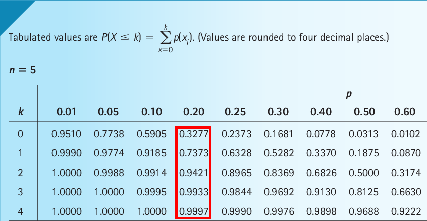
For \(n=5\) and \(p=0.2\), we see from the table that

• \(P(X \le 0) = P(X = 0) = 0.3277\)
• \(P(X \le 1) = 0.7373\)
• \(P(X \le 2) = 0.9421\)
• \(P(X \le 3) = 0.9933\)
• \(P(X \le 4) = 0.9997\)
• \(P(X \le 5) = 1\), which is obvious, so there is no need to make a cell for it in the table
• \(P(X < 3) = P[X \le (3-1)] = P(X \le 2) = 0.9421\)
• \(P(X \ge 3) = 1 - P[X \le (3 - 1)] = 1 - P(X \le 2) = 1 - 0.9421 = 0.0579\)
• \(P(X > 3) = 1 - P(X \le 3) = 1 - 0.9933 = 0.0067\)
• \(P(X = 3) = P(X \le 3) - P[X \le (3 - 1)] = P(X \le 3) - P(X \le 2) = 0.9933 - 0.9421 = 0.0512\)
• \(P(2 < X < 5) = P[X \le (5 - 1)] - P(X \le 2) = P(X \le 4) - P(X \le 2) = 0.9997 - 0.9421 = 0.0576\)
• \(P(2 \le X < 5) = P[X \le (5 - 1)] - P[X \le (2 - 1)] = P(X \le 4) - P(X \le 1) = 0.9997 - 0.7373 = 0.2624\)
• \(P(2 < X \le 5) = P(X \le 5) - P(X \le 2) = 1 - 0.9421 = 0.0579\)
• \(P(2 \le X \le 5) = P(X \le 5) - P[X \le (2 - 1)] = P(X \le 5) - P(X \le 1) = 1 - 0.7373 = 0.2627\)

Example

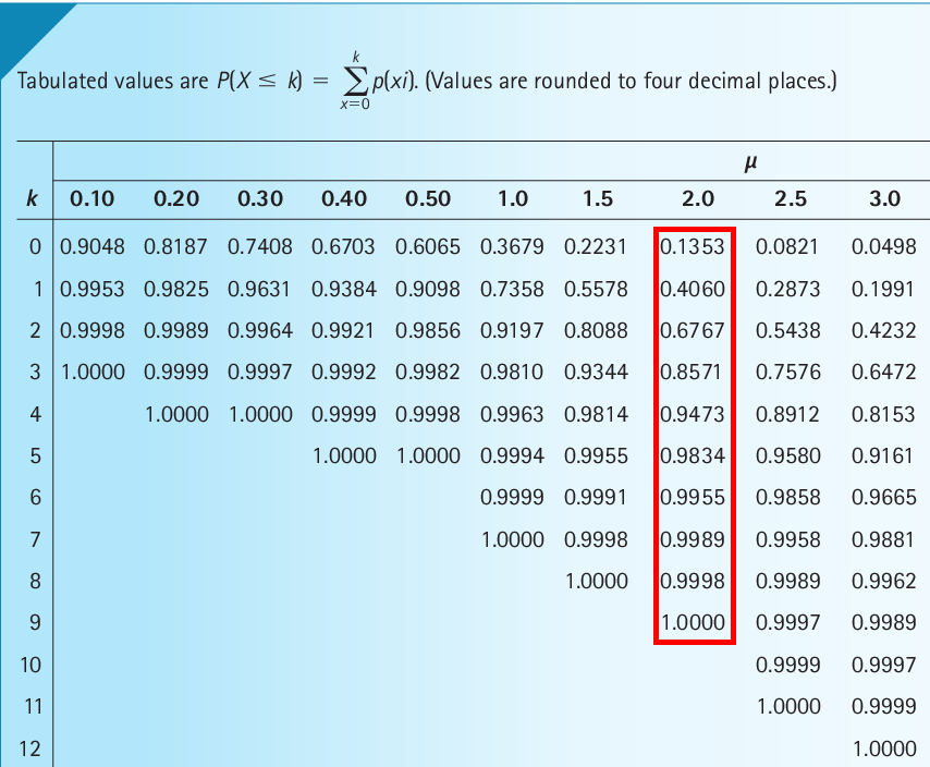
For \(\mu = 3\),

• \(P(X \le 0) = P(X = 0) = 0.1353\)
• \(P(X \le 1) = 0.4060\)
• \(P(X \le 2) = 0.6767\)
• \(P(X \le 3) = 0.8571\)
• \(P(X \le 4) = 0.9473\)
• \(P(X \le 5) = 0.9834\)
• \(\dots\)
• \(P(X < 3) = P[X \le (3-1)] = P(X \le 2) = 0.6767\)
• \(P(X \ge 3) = 1 - P[X \le (3 - 1)] = 1 - P(X \le 2) = 1 - 0.6767 = 0.3233\)
• \(P(X > 3) = 1 - P(X \le 3) = 1 - 0.8571 = 0.1429\)
• \(P(X = 3) = P(X \le 3) - P[X \le (3 - 1)] = 0.8571 - 0. 6767 = 0.1804\)
• \(P(2 < X < 5) = P[X \le (5 - 1)] - P(X \le 2) = P(X \le 4) - P(X \le 2) = 0.9473 - 0.6767 = 0.2706\)
• \(P(2 \le X < 5) = P[X \le (5 - 1)] - P[X \le (2 - 1)] = P(X \le 4) - P(X \le 1) = 0.9473 - 0.4060 = 0.5413\)
• \(P(2 < X \le 5) = P(X \le 5) - P(X \le 2) = 0.9834 - 0.6767 = 0.3067\)
• \(P(2 \le X \le 5) = P(X \le 5) - P[X \le (2 - 1)] = P(X \le 5) - P(X \le 1) = 0.9834 - 0.4060 = 0.5774\)