STAT 3360 Notes

1. Probability of Events
2. References

1 Probability of Events

1.1 Notation

We use \(P(A)\) to indicate the probability of an event \(A\).

1.2 Probability of Events

1.2.1 Definition

The formal definition of probability is too technical, so we don't discuss it in this course.
We define the probability of a simple event = the relative frequency of this simple event over the whole population.
We define the probability of a general event = the sum of the probabilities of all simple events constituting this event.

1.2.2 Examples

For example, suppose we there are \(200\) students in STAT 3360 in total and we regard them as the population. If \(24\) of these students are tall and and \(16\) are short, then
- \(P\)(the student is tall) = \(\frac{24}{200} = 12\%\), (probability of a simple event)
- \(P\)(the student is short) = \(\frac{16}{200} = 8\%\), (probability of a simple event)
- \(P\)(the student is tall or short) = \(P\)(the student is tall) + \(P\)(the student is short) = \(\frac{24}{200} + \frac{16}{200}= 20\%\), (probability of a general event)

1.3 Probability: One Variable

1.3.1 Simple Event: Distribution Table

If an experiment about a single variable has a finite number of outcomes, then the probabilities of all simple events can be given by a Distribution Table.
For example, if the experiment is about a single variable Height, then we may express the probabilities of all simple events in the following distribution table

Height Tall Medium Short Total

Probability \(12\%\) \(80\%\) \(8\%\) \(100\%\)

From the above table, we know the following probabilities of simple events
- \(P\)(height = tall) = \(12\%\)
- \(P\)(height = medium) = \(80\%\)
- \(P\)(height = short) = \(8\%\)
For example, if the experiment is about a single variable Weight, then we may express the probabilities of all simple events in the following distribution table

Weight Heavy Medium Light Total

Probability \(5\%\) \(73\%\) \(22\%\) \(100\%\)

From the above table, we know the following probabilities of simple events
- \(P\)(weight = heavy) = \(5\%\)
- \(P\)(weight = medium) = \(73\%\)
- \(P\)(weight = light) = \(22\%\)

Height	Tall	Medium	Short	Total
Probability	\(12\%\)	\(80\%\)	\(8\%\)	\(100\%\)

Weight	Heavy	Medium	Light	Total
Probability	\(5\%\)	\(73\%\)	\(22\%\)	\(100\%\)

1.3.2 General Event

The probability of a general event is the sum of the probabilities of the simple events that constitute the event.
For experiment about a single variable, the probability of each simple event can be found in the distribution table.
For example, if the experiment is about a single variable Height, then we use the distribution table of Height and get
- \(P\)(height = tall or short)
  
  = \(P\)(height = tall) + \(P\)(height = short) = \(12\% + 8\% = 20 \%\),
- \(P\)(height = at least medium) = \(P\)(height = medium or tall)
  
  = \(P\)(height = medium) + \(P\)(height = tall) = \(80\% + 12\% = 92\%\),
- \(P\)(height = at most medium) = \(P\)(height = medium or short)
  
  = \(P\)(height = medium) + \(P\)(height = short) = \(80\% + 8\% = 88\%\),
Height Tall Medium Short Total

Probability \(12\%\) \(80\%\) \(8\%\) \(100\%\)

Height	Tall	Medium	Short	Total
Probability	\(12\%\)	\(80\%\)	\(8\%\)	\(100\%\)

1.4 Probability: Two Variables

1.4.1 Simple Event: Joint Distribution Table

If an experiment about two (or more) variables has a finite number of outcomes, then the probabilities of all simple events can be given by a Joint Distribution Table.
In the joint distribution table, each cell shows the probability of the corresponding simple event of the experiment about the two variables.
For example, if the experiment is about both Height and Weight, then we may express the probabilities of all simple events in the following joint distribution table

Probability Heavy Medium Light

Tall \(0\%\) \(12\%\) \(0\%\)

Medium \(5\%\) \(59\%\) \(16\%\)

Short \(0\%\) \(2\%\) \(6\%\)

From the above table, we know the following probabilities of simple events
- \(P\)(height = tall and weight = heavy) = \(0\%\)
- \(P\)(height = tall and weight = medium) = \(12\%\)
- \(P\)(height = tall and weight = light) = \(0\%\)
- \(P\)(height = medium and weight = heavy) = \(5\%\)
- \(P\)(height = medium and weight = medium) = \(59\%\)
- \(P\)(height = medium and weight = light) = \(16\%\)
- \(P\)(height = short and weight = heavy) = \(0\%\)
- \(P\)(height = short and weight = medium) = \(2\%\)
- \(P\)(height = short and weight = light) = \(6\%\)

Probability	Heavy	Medium	Light
Tall	\(0\%\)	\(12\%\)	\(0\%\)
Medium	\(5\%\)	\(59\%\)	\(16\%\)
Short	\(0\%\)	\(2\%\)	\(6\%\)

1.4.2 General Event

The probability of a general event is the sum of the probabilities of the simple events that constitute the event.
For experiment about two (or more) variables, the probability of each simple event can be found in the joint distribution table.

For example, if the experiment is about two variables Height and Weight, then we use the joint distribution table of Height and Weight and get

\(P\)(height = tall or weight = heavy)

= \(P\)(height = tall and weight = heavy)

+\(P\)(height = tall and weight = medium)

+\(P\)(height = tall and weight = light)

+\(P\)(height = medium and weight = heavy)

+\(P\)(height = short and weight = heavy)

= \(0\% + 12\% + 0\% + 5\% + 0\% = 17\%\)

Probability Heavy Medium Light

Tall \(\boxed{0\%}\) \(\boxed{12\%}\) \(\boxed{0\%}\)

Medium \(\boxed{5\%}\) \(59\%\) \(16\%\)

Short \(\boxed{0\%}\) \(2\%\) \(6\%\)
\(P\)(height = tall and weight = not heavy)

= \(P\)(height = tall and weight = medium) + \(P\)(height = tall and weight = light)

= \(12\% + 0\% = 12\%\)

Probability Heavy Medium Light

Tall \(0\%\) \(\boxed{12\%}\) \(\boxed{0\%}\)

Medium \(5\%\) \(59\%\) \(16\%\)

Short \(0\%\) \(2\%\) \(6\%\)

\(P\)(height = tall or weight = not heavy)

= \(P\)(height = tall and weight = heavy)

+\(P\)(height = tall and weight = medium)

+\(P\)(height = tall and weight = light)

+\(P\)(height = medium and weight = medium)

+\(P\)(height = medium and weight = light)

+\(P\)(height = short and weight = medium)

+\(P\)(height = short and weight = light)

= \(0\% + 12\% + 0\% + 59\% + 16\% + 2\% + 6\% = 95\%\)

Probability	Heavy	Medium	Light
Tall	\(\boxed{0\%}\)	\(\boxed{12\%}\)	\(\boxed{0\%}\)
Medium	\(5\%\)	\(\boxed{59\%}\)	\(\boxed{16\%}\)
Short	\(0\%\)	\(\boxed{2\%}\)	\(\boxed{6\%}\)

\(P\)(height = not tall and weight = not heavy)

= \(P\)(height = medium and weight = medium) + \(P\)(height = medium and weight = light)

+\(P\)(height = short and weight = medium) + \(P\)(height = short and weight = light)

= \(59\% + 16\% + 2\% + 6\% = 83\%\)

Probability Heavy Medium Light

Tall \(0\%\) \(12\%\) \(0\%\)

Medium \(5\%\) \(\boxed{59\%}\) \(\boxed{16\%}\)

Short \(0\%\) \(\boxed{2\%}\) \(\boxed{6\%}\)

Probability	Heavy	Medium	Light
Tall	\(0\%\)	\(12\%\)	\(0\%\)
Medium	\(5\%\)	\(\boxed{59\%}\)	\(\boxed{16\%}\)
Short	\(0\%\)	\(\boxed{2\%}\)	\(\boxed{6\%}\)

\(P\)(height = not tall or weight = not heavy)

= \(P\)(height = tall and weight = medium)

+\(P\)(height = tall and weight = light)

+\(P\)(height = medium and weight = heavy)

+\(P\)(height = medium and weight = medium)

+\(P\)(height = medium and weight = light)

+\(P\)(height = short and weight = heavy)

+\(P\)(height = short and weight = medium)

+\(P\)(height = short and weight = light)

= \(12\% + 0\% + 5\% + 59\% + 16\% + 0\% + 2\% + 6\% = 100\%\)

Probability	Heavy	Medium	Light
Tall	\(0\%\)	\(\boxed{12\%}\)	\(\boxed{0\%}\)
Medium	\(\boxed{5\%}\)	\(\boxed{59\%}\)	\(\boxed{16\%}\)
Short	\(\boxed{0\%}\)	\(\boxed{2\%}\)	\(\boxed{6\%}\)

1.5 Marginal Distribution

1.5.1 Definitions

If we are given only the joint distribution table of two variables, how to get the respective distribution table of each individual variable?
The row totals and column totals of the joint distribution table are called Marginal Probabilities.
By including the marginal probabilities, the joint distribution table can be augmented to the Joint and Marginal Distribution Table.
A row total represents the probabilitiy of the corresponding event of the column variable.
A column total represents the probabilitiy of the corresponding event of the row variable.
The row header and all column totals form the distribution table of the row variable.
The column header and all row totals form the distribution table of the column variable.

1.5.2 Example

The experiment about both Height and Weight has the following joint distribution table

Probability Heavy Medium Light

Tall \(0\%\) \(12\%\) \(0\%\)

Medium \(5\%\) \(59\%\) \(16\%\)

Short \(0\%\) \(2\%\) \(6\%\)

Probability	Heavy	Medium	Light
Tall	\(0\%\)	\(12\%\)	\(0\%\)
Medium	\(5\%\)	\(59\%\)	\(16\%\)
Short	\(0\%\)	\(2\%\)	\(6\%\)

We can calculate the row totals and column totals of the joint distribution table

Probability	Heavy	Medium	Light	Row Total
Tall	\(0\%\)	\(12\%\)	\(0\%\)	\(\boxed{12\%}\)
Medium	\(5\%\)	\(59\%\)	\(16\%\)	\(\boxed{80\%}\)
Short	\(0\%\)	\(2\%\)	\(6\%\)	\(\boxed{8\%}\)
Column Total	\(\boxed{5\%}\)	\(\boxed{73\%}\)	\(\boxed{22\%}\)	\(\boxed{100\%}\)

The row totals and column totals are called Marginal Probabilities, and this augmented table is called the Joint and Marginal Probability Table

Probability	Heavy	Medium	Light	\(\boxed{\textbf{Marginal}}\)
Tall	\(0\%\)	\(12\%\)	\(0\%\)	\(12\%\)
Medium	\(5\%\)	\(59\%\)	\(16\%\)	\(80\%\)
Short	\(0\%\)	\(2\%\)	\(6\%\)	\(8\%\)
\(\boxed{\textbf{Marginal}}\)	\(5\%\)	\(73\%\)	\(22\%\)	\(100\%\)

A row total represents the probabilitiy of the corresponding event of the column variable Height, and a column total represents the probabilitiy of the corresponding event of the row variable Weight.

Probability	Heavy	Medium	Light	Marginal
Tall	\(0\%\)	\(12\%\)	\(0\%\)	\(P\)(height = tall) = \(12\%\)
Medium	\(5\%\)	\(59\%\)	\(16\%\)	\(P\)(height = medium) = \(80\%\)
Short	\(0\%\)	\(2\%\)	\(6\%\)	\(P\)(height = short) = \(8\%\)
Marginal	\(P\)(weight = heavy) = \(5\%\)	\(P\)(weight = medium) = \(73\%\)	\(P\)(weight = light) = \(22\%\)	\(100\%\)

The row header and all column totals form the distribution table of the row variable Weight

Weight Heavy Medium Light Total

Probability \(5\%\) \(73\%\) \(22\%\) \(100\%\)
The column header and all row totals form the distribution table of the column variable Height

Height Tall Medium Short Total

Probability \(12\%\) \(80\%\) \(8\%\) \(100\%\)

Weight	Heavy	Medium	Light	Total
Probability	\(5\%\)	\(73\%\)	\(22\%\)	\(100\%\)

Height	Tall	Medium	Short	Total
Probability	\(12\%\)	\(80\%\)	\(8\%\)	\(100\%\)

1.6 Independence of Events

1.6.1 Defintion

Two events A and B are called Independent if \[ \boxed{ P(A \text{ and } B) = P(A) P(B) }\]

1.6.2 Example

For example, from the joint and marginal distribution tables of Height and Weight, we know

\(P\)(height = short) = \(8\%\)
\(P\)(weight = light) = \(22\%\)
\(P\)(height = short) \(\cdot\) \(P\)(weight = light) = \(8\% \cdot 22 \% = 1.76\%\)
\(P\)(heigh = short and weight = light) = \(6\%\)

Since \(1.76\% \neq 6\%\), the two events "height = short" and "weight = light" are not independent. Intuitively, a shorter person tend to be lighter.

Probability	Heavy	Medium	Light	Marginal
Tall	\(0\%\)	\(12\%\)	\(0\%\)	\(P\)(height = tall) = \(12\%\)
Medium	\(5\%\)	\(59\%\)	\(16\%\)	\(P\)(height = medium) = \(80\%\)
Short	\(0\%\)	\(2\%\)	\(6\%\)	\(P\)(height = short) = \(8\%\)
Marginal	\(P\)(weight = heavy) = \(5\%\)	\(P\)(weight = medium) = \(73\%\)	\(P\)(weight = light) = \(22\%\)	\(100\%\)

1.7 Complement Rule

1.7.1 The Rule

For any event \(A\), \[ \boxed{ P(A^C) = 1 - P(A)} \]

1.7.2 Example

For example, in the experiment about a single variable Height,
- \(P\)(height = not tall)
  
  = \(1 - P\)(height = tall)
  
  = \(1- 12\% = 88\%\),
- \(P\)[height = neither tall nor short]
  
  = \(1 - P\)(height = either tall or short)
  
  = \(1 -\) [\(P\)(height = tall) + \(P\)(height = short)]
  
  = \(1 - (12\% + 8\%) = 80\%\),
- \(P\)(height = at least medium)
  
  = \(1 - P\)(height = shorter than medium)
  
  = \(1 - P\)(height = short)
  
  = \(1 - 8\% = 92\%\),
- \(P\)(height = at most medium)
  
  = \(1 - P\)(height = taller than medium)
  
  = \(1 - P\)(height = tall)
  
  = \(1 - 12\% = 88\%\).
For example, in the experiment about both Height and Weight,
- \(P\)(the student is not tall or not heavy)
  
  = \(1 - P\)(the student is both tall and heavy)
  
  = \(1- 0\% = 100\%\),
  
  Probability Heavy Medium Light
  
  Tall \(\boxed{0\%}\) \(12\%\) \(0\%\)
  
  Medium \(5\%\) \(59\%\) \(16\%\)
  
  Short \(0\%\) \(2\%\) \(6\%\)
- \(P\)(the student is either tall or heavy)
  
  = \(1 - P\)(the student is neither tall nor heavy)
  
  = \(1 - (59\% + 16\% + 2\% + 6\%)\)
  
  = \(1- 83\% = 17\%\),
  
  Probability Heavy Medium Light
  
  Tall \(0\%\) \(12\%\) \(0\%\)
  
  Medium \(5\%\) \(\boxed{59\%}\) \(\boxed{16\%}\)
  
  Short \(0\%\) \(\boxed{2\%}\) \(\boxed{6\%}\)

Probability	Heavy	Medium	Light
Tall	\(\boxed{0\%}\)	\(12\%\)	\(0\%\)
Medium	\(5\%\)	\(59\%\)	\(16\%\)
Short	\(0\%\)	\(2\%\)	\(6\%\)

Probability	Heavy	Medium	Light
Tall	\(0\%\)	\(12\%\)	\(0\%\)
Medium	\(5\%\)	\(\boxed{59\%}\)	\(\boxed{16\%}\)
Short	\(0\%\)	\(\boxed{2\%}\)	\(\boxed{6\%}\)

1.8 Addition Rule

1.8.1 The Rule

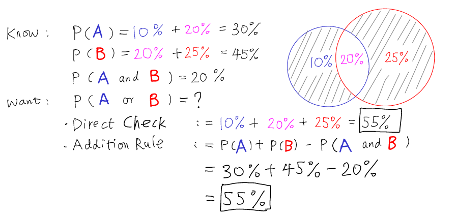
For any event A and any event B, \[ \boxed {P(A \text{ or } B) = P(A) + P(B) - P(A \text{ and } B) } \] and thus \[ \boxed {P(A \text{ and } B) = P(A) + P(B) - P(A \text{ or } B) } \] Note: This rule connects intersection and union of the two events.

1.8.2 Example

if \(P\)(A) = \(30\%\), \(P\)(B) = \(40\%\) and \(P\)(A and B) = \(20\%\), then

\(P\)(A or B) = \(P\)(A) + \(P\)(B) - \(P\)(A and B)

= \(30\% + 40\% - 20\% = 50\%\)
if \(P\)(A) = \(30\%\), \(P\)(B) = \(40\%\) and \(P\)(A or B) = \(50\%\), then

\(P\)(A and B) = \(P\)(A) + \(P\)(B) - \(P\)(A or B)

= \(30\% + 40\% - 50\% = 20\%\)
if A = "the student is tall" and B = "the student is short", then we have

\(P\)(A or B) = \(P\)(A) + \(P\)(B) - \(P\)(A and B)

= \(P\)(height = tall) + \(P\)(height = short) - \(P\)(height = tall and short)

= \(12\% + 8\% - 0\% = 20\%\).

Height Tall Medium Short Total

Probability \(12\%\) \(80\%\) \(8\%\) \(100\%\)

Height	Tall	Medium	Short	Total
Probability	\(12\%\)	\(80\%\)	\(8\%\)	\(100\%\)

if A = "the student is short" and B = "the student is light", then we have

\(P\)(A or B) = \(P\)(A) + \(P\)(B) + \(P\)(A and B)

= \(P\)(height = short) + \(P\)(weight = light) - \(P\)(height = short and weight = light)

= \(8\% + 22\% - 6\% = 24\%\).

Probability	Heavy	Medium	Light	Marginal
Tall	\(0\%\)	\(12\%\)	\(0\%\)	\(P\)(height = tall) = \(12\%\)
Medium	\(5\%\)	\(59\%\)	\(16\%\)	\(P\)(height = medium) = \(80\%\)
Short	\(0\%\)	\(2\%\)	\(6\%\)	\(P\)(height = short) = \(8\%\)
Marginal	\(P\)(weight = heavy) = \(5\%\)	\(P\)(weight = medium) = \(73\%\)	\(P\)(weight = light) = \(22\%\)	\(100\%\)

1.9 Conditional Probability

1.9.1 Introduction

What is the probability that a student goes to men's restroom? Maybe \(50\%\).
What is the probability that a student goes to men's restroom, if the student is a male? It should be \(100\%\).
The probability of the same event "a student goes to men's restroom" changes from \(50\%\) to \(100\%\), because the popultion of interest has changed from "all students" to "all male students".
Generally, when a condition is given, the population of interest changes and thus the probability of the event also changes, as shown above. This is the reason why we introduce the conditional probability.

1.9.2 Definition

The probability of event A given event B is defined as \[ \boxed{ P(A|B) = \frac{P(A \text{ and } B)}{P(B)} } \]
The probability of event B given event A is defined as \[ \boxed{ P(B|A) = \frac{P(A \text{ and } B)}{P(A)} } \]
If A and B are independent, then \(P\)(A and B) = \(P\)(A)\(P\)(B) and thus \(P\)(A | B) = \(P\)(A) and \(P\)(B | A) = \(P\)(B). That is, the conditional probabilities are equal to the "unconditional" ones, which is just the literal meaning of "independence".

1.9.3 Example

For example, for the experiment about both Height and Weight, we have

\(P\)(weight = light|height = short) = \(\frac{P(\text{weight = light and height = short})}{P(\text{height = short})} = \frac{6\%}{8\%} = 75\%\).

That is to say, when a student is short, it is \(75\%\) likely that he/she is also light. Without the condition "the student is short", it is only \(22\%\) likely that a student is light (the marginal probability). This shows the difference between the conditional probability and unconditional probability.

Probability	Heavy	Medium	Light	Marginal
Tall	\(0\%\)	\(12\%\)	\(0\%\)	\(P\)(height = tall) = \(12\%\)
Medium	\(5\%\)	\(59\%\)	\(16\%\)	\(P\)(height = medium) = \(80\%\)
Short	\(0\%\)	\(2\%\)	\(6\%\)	\(P\)(height = short) = \(8\%\)
Marginal	\(P\)(weight = heavy) = \(5\%\)	\(P\)(weight = medium) = \(73\%\)	\(P\)(weight = light) = \(22\%\)	\(100\%\)

1.10 Multiplication Rule

From the definition of conditional probability, we immediately have

for any event A and any event B \[ \boxed{ P(A \text{ and } B) = P(A) P(B|A) } \] \[ \boxed{ P(A \text{ and } B) = P(B) P(A|B) } \]

1.11 Probability Tree

1.11.1 Why and When

When discussing two (or more) variables at the same time, we have joint probabilities, marginal probabilities and conditional probabilities. Probability tree is a helpful tool for visualizing these probabilities.

1.11.2 How to Draw

Suppose
- the first variable \(X\) has \(k\) different values \(u_1, u_2, \dots, u_r\),
- the second variable \(Y\) has \(l\) different values \(v_1, v_2, \dots, v_s\),

To draw the probability tree using \(X\) as the first step and \(Y\) as the second step,

Make the Marginal and Conditional Probability Table. If the table is already given, then skip this step.

X	u₁	u₂	…	u_r
Marginal Probability	P(X=u₁)	P(X=u₂)	…	P(X=u_r)
Conditional Probability of Y=v₁	P(Y=v₁\(\vert\) X=u₁)	P(Y=v₁\(\vert\) X=u₂)	…	P(Y=v₁\(\vert\) X=u_r)
Conditional Probability of Y=v₂	P(Y=v₂\(\vert\) X=u₁)	P(Y=v₂\(\vert\) X=u₂)	…	P(Y=v₂\(\vert\) X=u_r)
…	…	…	…	…
Conditional Probability of Y=v_s	P(Y=v_s\(\vert\) X=u₁)	P(Y=v_s\(\vert\) X=u₂)	…	P(Y=v_s\(\vert\) X=u_r)

Draw a single dot as the root.
From the root, draw \(r\) branches for the first variable \(X\),
Then the \(i\)-th branch from the root represents a simple event \(X=u_i\) and we can write down its probability \(P(X=u_i)\),
From the \(i\)-th branch, draw \(s\) sub-branches for the second variable \(Y\),
Then the \(j\)-th sub-branch from the \(i\)-th branch represents the event \(Y=v_j\) given \(X=u_i\) and we can write down the its probability \(P(Y=v_j | X=u_i)\)
The end (leaf) of the \(j\)-th sub-branch from the \(i\)-th branch represents the intersection of event \(X=u_i\) and \(Y=v_j\) and we can write down its probability by the multiplication rule \(P(X = u_i \text{ and } Y = v_j) = P(X = u_i) \times P(Y = v_j | X = u_i)\).
If needed, put the joint probabilities into a joint distribution table.

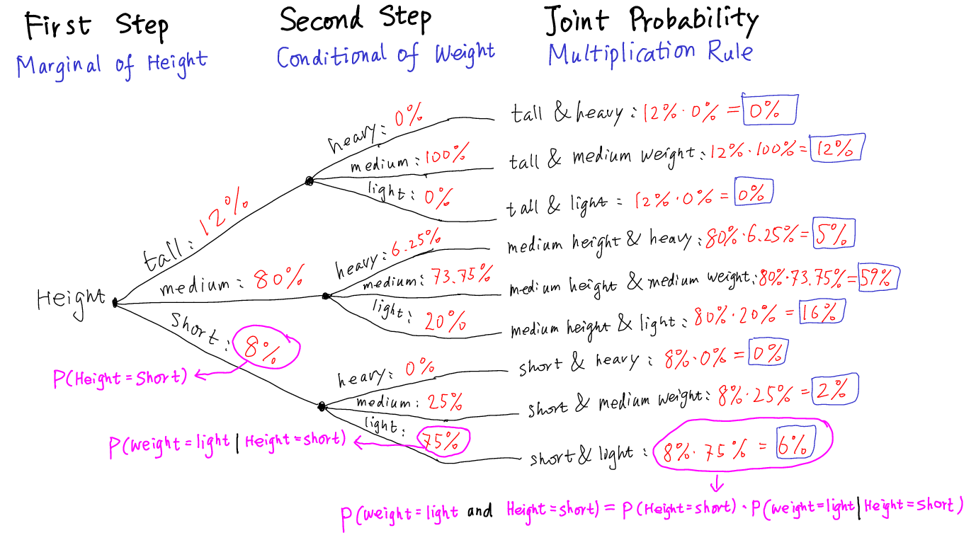
1.11.3 Example

Let's still use the height and weight example. Draw a probability tree
- using height as the first step (\(X\)), and
- using weight as the second step (\(Y\)).

Make the conditional probability table.

The values of \(X\) (height) are tall, medium and short,
The values of \(Y\) (weight) are heavy, medium and light,

Then the conditional probability table has the form

\(X\) (Height)	Tall (T)	Medium (MH)	Short (S)
Marginal Probability	P(X=T)	P(X=MH)	P(X=S)
Cond. Prob. of \(Y\) = Heavy(H)	P(Y=H \| X=T)	P(Y=H \| X=MH)	P(Y=H \| X=S)
Cond. Prob. of \(Y\) = Medium(MW)	P(Y=MW \| X=T)	P(Y=MW \| X=MH)	P(Y=MW \| X=S)
Cond. Prob. of \(Y\) = Light(L)	P(Y=L \| X=T)	P(Y=L \| X=MH)	P(Y=L \| X=S)

Find the probabilities in the table. For example, from the joint and marginal distribution table of Height and Weight, we know

\(P\)(height = tall) = \(12\%\)
\(P\)(weight = medium | height = short) = \(\frac{P(\text{weight = medium and height = short})}{P(\text{height = short})} = \frac{2\%}{8\%} = 25\%\).

\(X\) (Height)	Tall	Medium	Short
Marginal Probability	\(12\%\)	\(80\%\)	\(8\%\)
Conditional Probability of \(Y\) = Heavy	\(0\%\)	\(6.25\%\)	\(0\%\)
Conditional Probability of \(Y\) = Medium	\(100\%\)	\(73.75\%\)	\(25\%\)
Conditional Probability of \(Y\) = Light	\(0\%\)	\(20\%\)	\(75\%\)

Draw the probability tree

1.12 Solving Word Problems

IDENTIFY THE PROBLEM!
- What is the experiment? Is it about a single variable or two variables? What is (are) the variabale(s) of interest?
- What are the outcomes of the experiment? What are the values of the variable(s)?
- Is the problem about probability of a simple event or general event?
- Is the problem about an intersection event, a union event, or a complement event?
- How to translate terms like "at most" or "at least"?
- And so forth.
WRITE DOWN THE DISTRIBUTION TABLES!
- As we see, Distribution Table (for a single variable) and Joint and Marginal Distribution Table (for two variables) are the foundation for ALL further calculations (probability of simple event, general event, complement event, union event and intersection event, conditional probability and probability tree).
APPLY THE CORRECT RULES AND TECHNIQUES!
- Once you have identified the nature of the problem and have got the necessary tables, think of relevent rules and technqiues for solving the problem.

2 References

Keller, Gerald. (2015). Statistics for Management and Economics, 10th Edition. Stamford: Cengage Learning.