STAT 3360 Notes
Table of Contents
1 Relationship between Interval Variables
1.1 Raw Data: Student Weight and Height
Let's use the full Student Weight and Height data. For simplicity, observations are rounded to integers, but all notions and techniques introduced in this section can be applied to non-integers in exactly the same way.
StudentID Height Weight StudentID Height Weight StudentID Height Weight 1 66 113 18 66 130 35 72 140 2 72 136 19 69 143 36 69 129 3 69 153 20 71 138 37 67 142 4 68 142 21 67 124 38 68 121 5 68 144 22 68 141 39 68 131 6 69 123 23 69 144 40 64 107 7 70 141 24 63 98 41 69 124 8 70 136 25 68 130 42 65 125 9 68 112 26 68 142 43 70 140 10 67 121 27 67 130 44 68 137 11 66 127 28 71 142 45 66 106 12 68 114 29 67 132 46 69 129 13 68 126 30 67 108 47 67 146 14 67 122 31 65 114 48 68 117 15 68 116 32 70 103 49 70 144 16 71 140 33 66 121 50 69 135 17 66 130 34 68 126 51 70 147
1.2 Introduction
- For the data of each individual interval variable, we have already learned measures of central location, variability and relative standing.
- In many cases, for each subject in the population, we are interested in more than one of its characteristics, so we may consider multiple variables simultaneously. For example, for each student, we are interested in both Height and Weight of the student, so we define the two variables at the same time and get data for both of them, as above.
- Intuitively, since we observe both Weight and Height from the same student, we may believe there is some (linear) relationship between them. For example, if a student is tall, then there is a high chance that the student is also heavy.
- Therefore, we should consider two interval variables together, and
- measure the relationship between them (for simplicity, only linear relationship is considered),
- Predict the value of one variable if we know the value of the other.
1.3 Bivariate Data
- When considering the relationship between two variables, we always use the "matched" data. That is, for any \(x\)-value in the data, only the \(y\)-value of the same subject is used. For example, we don't consider the relationship between Jack's weight and David's height.
1.4 Measures of Linear Relationship
1.4.1 Linear Relationship
- If the relationship between two variables \(X\) and \(Y\) can be expressed or approximated by \(Y = b_0 + b_1 X\) where \(b_0\) and \(b_1 \neq 0\) are constants, then we say there is a linear relationship between \(X\) and \(Y\).
- Geometrically, \(Y = b_0 + b_1 X\) means a straight line in the coordinate system, which is the reason why we call the relationship linear.
- For example, suppose \(Y\) and \(X\) are the Celsius and Fahrenheit measures of the same temperature respectively, then the relationship between them is \(Y = - \frac{160}{9} + \frac{5}{9} \cdot X\) where \(b_0 = - \frac{160}{9}\) and \(b_1 = \frac{5}{9}\). This is a perfect mathematical linear relationship without any randomness.
- In statistics, we seldom have perfect relationship between two variables. For example, we may say the relationship between weight \(Y\) and height \(X\) of a student is close to \(Y = −133 + 3.8X\), but we can't say this relationship is perfect. Obviously, even if we know the accurate height of a student is \(70\), we can't say the weight of the student is definitely \(-133 + 3.8 \cdot 70 = 133\). The weight of the student is not only related to the height, but also related to some other random factors. Once randomness takes place, the problem is not a mathematical one, but a statistical one, and we thus need statistical techniques to treat it.
1.4.2 Two-Variable Graph: Scatter Plot
- Introduction
- A scatter plot is used for illustrating the relationship between two interval variables.
- If there is a relationship between the two variables, then there should be a corresponding pattern in the plot.
- How to Draw a Scatter Plot
- Suppose we have the data of \(n\) subjects on two variables: \(\{ (x_1, y_1), (x_2, y_2), \dots, (x_n, y_n) \}\).
- use the values of the first variable \(X\) as the x-axis,
- use the values of the second variable \(Y\) as the y-axis,
- for the \(i\)-th subject, \(i=1,2,3,\dots,n\), draw a point using \(x_i\) as the \(x\)-coordinate and \(y_i\) as the \(y\)-coordinate.
- Example
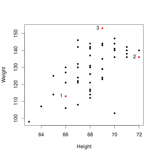
For the Student Weight and Height data, we can use Height as the x-axis and Weight as the y-axis, and get the following scatter plot
or, we can use Weight as the x-axis and Height as the y-axis, and get the following scatter plot
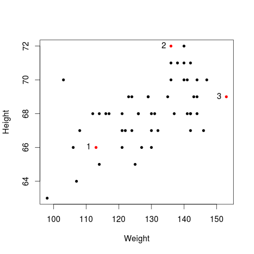
- Roughly speaking, a large value of Height is likely to mean a large value of Weight.
1.4.3 Sample Covariance
- Suppose we have the data of \(n\) subjects on two variables \(X\) and \(Y\): \(\{ (x_1, y_1), (x_2, y_2), \dots, (x_n, y_n) \}\).
- Then the sample covariance \(s_{xy}\) is defined as \[ \boxed{ s_{xy} = \frac{\sum\limits_{i=1}^{n}[(x_i-\bar{x})(y_i-\bar{y})]}{n-1} } \]
- The variance of a sample can be regarded as the coveriance between the sample and itself: \[ s_x^2 = s_{xx} = \frac{\sum\limits_{i=1}^{n}[(x_i-\bar{x})(x_i-\bar{x})]}{n-1} = \frac{\sum\limits_{i=1}^{n}(x_i-\bar{x})^2}{n-1} \]
- For the Student Weight and Height data, if we let variable \(X\) be the Height and let variable \(Y\) be the Weight, then
- The sample mean of Height is \(\bar{x} = \frac{66+72+69+\cdots+70}{51} = 68.14\)
- The sample mean of Weight is \(\bar{y} = \frac{113+136+153+\cdots+147}{51} = 129.18\)
- the covariance between Weight and Height is \(s_{xy} = \frac{(66-68.14)(113-129.18) + (72-68.14)(136-129.18) + (69-68.14)(153-129.18)+\cdots+(70-68.14)(147-129.18)}{51-1} = 14.32\)
1.4.4 Sample Coefficient of Correlation
- The sample coefficient of correlation between two variables \(X\) and \(Y\), denoted by \(r_{xy}\), is defined as the covariance (\(s_{xy}\)) divided by the standard deviations of both variables (\(s_x\) and \(x_y\)), that is,
\[ \boxed{ r_{xy} = \frac{s_{xy}}{s_x s_y} } \]
- \(-1 \le r_{xy} \le 1\) always holds.
- The larger the \(|r_{xy}|\) is, the stronger the linear relationship between the two variables is.
- Note that the coefficient of correlation only measures linear relationship between two variables. It is completely possible that there is a strong non-linear relationship between two variables but the \(|r_{xy}|\) is quite small or even \(0\).
- A positive value of \(r_{xy}\) means a trend such that as the value of the first variable increases, the value of the second variable is likely (not "certainly") to increase as well.
- A negative value of \(r\) means a trend such that as the value of the first variable increases, the value of the second variable is likely (not "certainly") to decrease.
- \(r=0\) means the two variables are linearly uncorrelated. However, as stated above, "linearly uncorrelated" does not mean "independent" or "not related at all".
- For the Student Weight and Height data, if we let variable \(X\) be the Height and let variable \(Y\) be the Weight,
- the variance of Height is \(s_x^2 = \frac{(113-129.18)^2 + (136-129.18)^2 + (153-129.18)^2 + \cdots (147-129.18)^2}{51-1} = 169.87\) and thus the standard deviation is \(s_x = \sqrt{s_x^2} = \sqrt{169.87} = 13.03\),
- the variance of Weight is \(s_y^2 = \frac{(66-68.14)^2 + (72-68.14)^2 + (69-68.14)^2 + \cdots (70-68.14)^2}{51-1} = 3.72\) and thus the standard deviation is \(s_y = \sqrt{s_y^2} = \sqrt{3.72} = 1.93\),
- the coefficient of correlation between Weight and Height is \(r_{xy} = \frac{14.32}{1.93\cdot 13.03} = 0.57\).
1.5 Simple Linear Regression
1.5.1 Introduction
- Suppose there is a strong linear relationship between two variables, can we guess the value of one variable if we know the value of the other, or can we utilize the linear relationship? Intuitively, the answer is yes. How? Although coefficient of correlation measures the strength of the linear relationship, it doesn't directly help us with the guess. Instead, the Simple Linear Regression model can be used.
1.5.2 The Model
- As stated above, if there is a linear relationship between varaibles \(X\) and \(Y\), then \(Y\) can be approximated by a linear function of \(X\). That is, we can represent \(Y\) by \[ \boxed{ Y = b_0 + b_1 X} \] using intercept \(b_0\) and slope \(b_1\).
- Once \(b_0\) and \(b_1\) are known, for a given value of \(X\), we can immediately get the corresponding value of \(Y\) by direct substitution. For example, if we know \(b_0 = -133\) and \(b_1 = 3.8\), then for \(x=70\), we have \(y = -133 + 3.8 \times 70 = 133\).
1.5.3 Estimating the Coefficients
- In reality, due to various reasons, our observations of \(X\) and \(Y\) usually don't form a perfect straight line, as shown by the scatter plot. Therefore, we don't know the true values of \(b_0\) and \(b_1\) (actually, even if the observations form a perfect line, the intercept and slope are not necessarily the true values of \(b_0\) and \(b_1\)).
- What can we do if we want to know \(b_0\) and \(b_1\)? We can make a guess (called estimate in statistics) of them, say \(\hat{b}_0\) and \(\hat{b}_1\) respectively.
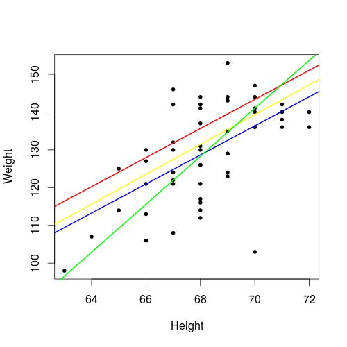
We can arbitrarily bring up our guess of \(b_0\) and \(b_1\), and there are thus infinitely many guesses \(\hat{b}_0\) and \(\hat{b}_1\). Then which one should we choose? Or which one is "the best", if any? As shown below, for the Student Weight and Height data, four possible straight lines are given, each of which corresponds to a specific combination of values of \(b_0\) and \(b_1\). Which line is the best? In some sense, the blue line is the best, because it corresponds to the so-called Least Squares Estimates discussed below.
1.5.4 Least Square Estimates of Coefficients
- Introduction
- As discussed above, for a given data, we would like to find "the best" straight line that best represents the the linear relationship between two interval variables \(X\) and \(Y\). In some sense, the best answer does exist, and is called Least Squares Estimates.
- Formula
- Suppose
- \(s_x^2\) is the sample variance of \(X\);
- \(s_{xy}\) is the sample covariance between \(X\) and \(Y\).
- Then the Least Squares Estimates of \(b_1\) and \(b_0\) are respectively \[ \boxed{\hat{b}_1 = \frac{s_{xy}}{s_x^2}} \] \[ \boxed{\hat{b}_0 = \bar{y} - \hat{b}_1 \bar{x}} \]
- Note:
- Find \(\hat{b}_1\) first, and then \(\hat{b}_0\).
- To find \(\hat{b}_1\), we use variance \(s_x^2\) and covariance \(s_{xy}\). If you are given standard deviation \(s_x\) or coefficient of correlation \(r_{xy}\) instead of \(s_x^2\) or \(s_{xy}\), then use the formulas \(s_x^2 = (s_x)^2\) and \(s_{xy} = r_{xy} s_x s_y\) to find them.
- Suppose
- Note
- As said before, least squares estimates is not the only choice for the estimate, although in some sense it is the best. The relevant criterion will be discussed later. If we use another criterion, then we may have another "best" estimate.
1.5.5 Fitted Model/Values/Line
- Once we have got specific estimates \(\hat{b}_0\) and \(\hat{b}_1\) (for example, the least squares estimates), we can put them into the equation \(Y = b_0 + b_1 X\) and get the estimated relationship between variables \(X\) and \(Y\), which is called the fitted model \[ \boxed{ Y = \hat{b}_0 + \hat{b}_1 X} \]
- For a specific value of variable \(X\), say \(x\), the fitted value \(\hat{y}\) for \(x\) is \[ \boxed{ \hat{y} = \hat{b}_0 + \hat{b}_1 x} \]
- If we connect all fitted values together, then they form a straight line, called the fitted line.
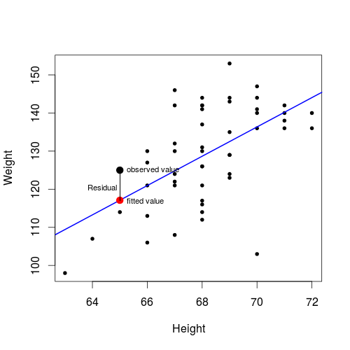
- In the plot below,
- the blue line represents our fitted line,
- each point on the fitted line represents a specific fitted value of weight for a given height,
- the big black point represents the observed height and weight of the 42th student,
the big red point represents our fitted value of this student, which is on the fitted line.
1.5.6 Residual
- The difference between the observed value \(y\) and the fitted value \(\hat{y}\) is called the residual \(e\), that is, \[ \boxed{ e = y - \hat{y} } \]
- Note: it is not \(\hat{y} - y\).
- \(e > 0\) means \(y > \hat{y}\) and thus the observed value is above the fitted value/line.
- \(e < 0\) means \(y < \hat{y}\) and thus the observed value is below the fitted value/line.
- \(e = 0\) means \(y = \hat{y}\) and thus the observed value overlaps the fitted value/line.
- \(e^2\) measures the distance between the observed value and the fitted value/line. The smaller the \(e^2\) is, the closer the fitted value is to the observed value and thus the better our estimates \(\hat{b}_0\) and \(\hat{b}_1\) are.
- In the plot above, the residual for the 42th student is shown.
1.5.7 Interpretation of Least Square Estimates
- Why are the Least Squares Estimates "the best"? Why are they given in that way?
- Suppose the observations of \((X, Y)\) are \((x_1, y_1), (x_2, y_2), \dots, (x_n, y_n)\). For any guess (not necessarily the Least Squares estimates) of \(\hat{b}_0\) and \(\hat{b}_1\),
- the fitted model is \(Y = \hat{b}_0 + \hat{b}_1 X\),
- the fitted value at \(x_i\), denoted by \(\hat{y}_i\), is \(\hat{y}_i = \hat{b}_0 + \hat{b}_1 x_i\),
- the residual at \(x_i\), denoted by \(e_i\), is \(e_i = y_i - \hat{y}_i = y_i - \hat{b}_0 - \hat{b}_1 x_i\),
- the residual sum of squares (RSS) over all observations is \(RSS = \sum\limits_{i=1}^{n} e_i^2 = \sum\limits_{i=1}^{n} (y_i - \hat{y}_i)^2 = \sum\limits_{i=1}^{n} (y_i - \hat{b}_0 - \hat{b}_1 x_i)^2\). By the definition \(RSS = \sum\limits_{i=1}^{n} e_i^2\), the RSS is large if \(e_i^2\) are large (ie, the fitted values are far from the observed values).
- Note that all \((x_i, y_i)\) pairs are the observations which are fixed numbers, so RSS is a function of only the estimates \(\hat{b}_0\) and \(\hat{b}_1\). Since the RSS measures the overall distance between the observed value and the fitted value, intuitively, we should choose \(\hat{b}_0\) and \(\hat{b}_1\) which make RSS as small as possible (so that the fitted values are close enough to the observed values).
- The estimates \(\hat{b}_0\) and \(\hat{b}_1\) which minimize the RSS is just called the Least Squares Estimate ("least" means "minimizing", and "squares" means RSS). The formula of least squares estimates is obtained using the technique learned in Calculus for finding the minimum of a function (RSS).
1.5.8 Example
For the Student Weight and Height data, if we let variable \(X\) be the Height and let variable \(Y\) be the Weight, then
- \(s_x^2 = 3.72\), as previously found
- \(s_{xy} = 14.32\), as previously found
- \(\bar{x} = 68.14\), as previously found
- \(\bar{y} = 129.18\), as previously found
- Thus the least squares estimates of \(b_1\) and \(b_0\) are
- \(\hat{b_1} = \frac{s_{xy}}{s_x^2} = \frac{14.32}{3.72} = 3.85\)
- \(\hat{b_0} = \bar{y} - \hat{b}_1 \bar{x} = 129.18 - 3.85 \cdot 68.14 = -133.16\)
- The fitted model is just \(\hat{Y} = -133.16 + 3.85\hat{X}\)
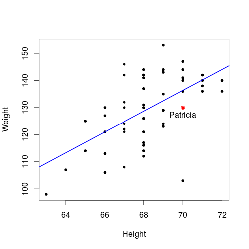
- Suppose the Height of Patricia is \(70\) inches, what is the estimate (fitted value) of her Weight?
- Here \(x=70\) and we want to estimate \(y\) for this \(x\). What we should do is just to let \(X = 70\) in the fitted model.
- Thus the estimate (fitted value) of Patricia's weight is \(\hat{y} = -133.16 + 3.85\cdot 70 = 136.34\).
- The true Weight of Patricia is \(130\) pounds. What is the residual for the above estimate of Patricia's weight?
- residual \(e = y - \hat{y} = 130 - 136.34 = -6.34\)
Is Patricia's record above or below the fitted line?
- since residual \(e=-6.34<0\), Patricia's record is below the fitted line.
2 References
- Keller, Gerald. (2015). Statistics for Management and Economics, 10th Edition. Stamford: Cengage Learning.