STAT 3360 Notes
Table of Contents
1 One-Population Inference: Population Mean
1.1 Population Standard Deviation Known
1.1.1 Assumptions and Notations
- \(X\): the random variable following a Normal distibution;
- \(\mu\): the unknown population mean of \(X\);
- \(\sigma\): the known population standard deviation of \(X\);
- \(X_1, X_2, \dots, X_n\): the sample of \(X\);
- \(n\): sample size;
- \(\bar{X}\): sample mean;
- \(s\): sample standard deviation;
- \(Z\): the standard Normal random variable;
- \(Z_{\alpha}\): the number such that \(P(Z > Z_{\alpha}) = \alpha\);
1.1.2 Confidence Interval
- This topic is already covered in a previous section titled "Estimating Population Mean". For completeness, let's repeat the relevant procedure and formulae here.
- When the population standard deviation of \(X\), denoted by \(\sigma\), is known, at Confidence Level \(1 - \alpha\), the Confidence Interval for the population mean \(\mu\) can be constructed as follows,
- Midpoint: \(\boxed{ \bar{X} }\);
- Critical Value: \(\boxed{ Z_{\alpha/2} }\);
- Margin of Error: \(\boxed{ Z_{\alpha/2} \cdot \frac{\sigma}{\sqrt{n}} }\);
- Lower Confidence Limit (LCL): \(\boxed{ \bar{X} - Z_{\alpha/2} \cdot \frac{\sigma}{\sqrt{n}} }\);
- Upper Confidence Limit (UCL): \(\boxed{ \bar{X} + Z_{\alpha/2} \cdot \frac{\sigma}{\sqrt{n}} }\);
- Confidence Interval: \(\boxed{ [\bar{X} - Z_{\alpha/2} \cdot \frac{\sigma}{\sqrt{n}}, \bar{X} + Z_{\alpha/2} \cdot \frac{\sigma}{\sqrt{n}}] }\);
- Width of Confidence Interval: \(\boxed{ 2 \cdot Z_{\alpha/2} \cdot \frac{\sigma}{\sqrt{n}} }\).
- At confidence level \(1-\alpha\), to achieve a confidence interval for the population mean \(\mu\) whose margin of error is no wider than \(M\), the smallest sample size needed is \[ \boxed{ n = \left( \frac{z_{\alpha/2} \sigma}{M} \right)^2 } \] If the value of \(n\) calculated by the formula is not an integer, then we should round it up in order to ensure the actual margin of error is no wider than \(M\).
1.1.3 Hypothesis Testing
- When the population standard deviation of \(X\), denoted by \(\sigma\), is known, at Significance Level \(\alpha\),
- the Z-test for \(\boxed{H_0: \mu \le \mu_0 \text{ vs } H_A: \mu > \mu_0}\) (which is equivalent to \(\boxed{H_0: \mu = \mu_0 \text{ vs } H_A: \mu > \mu_0}\)) can be constructed as follows,
- Test Statistic: \(\boxed{T = \frac{\sqrt{n}(\bar{X} - \mu_0)}{\sigma}}\);
- Critical Value: \(\boxed{Z_{\alpha}}\);
- Rejection Rule: Reject \(H_0\) if \(\boxed{T > Z_{\alpha}}\).
- the Z-test for \(\boxed{H_0: \mu \ge \mu_0 \text{ vs } H_A: \mu < \mu_0}\) (which is equivalent to \(\boxed{H_0: \mu = \mu_0 \text{ vs } H_A: \mu < \mu_0}\)) can be constructed as follows,
- Test Statistic: \(\boxed{T = \frac{\sqrt{n}(\bar{X} - \mu_0)}{\sigma}}\);
- Critical Value: \(Z_{1 - \alpha}\), which equals \(\boxed{- Z_{\alpha}}\);
- Rejection Rule: Reject \(H_0\) if \(T < Z_{1 - \alpha}\), which is equivalent to \(\boxed{T < -Z_{\alpha}}\).
- the Z-test for \(\boxed{H_0: \mu = \mu_0 \text{ vs } H_A: \mu \neq \mu_0}\) can be constructed as follows,
- Test Statistic: \(\boxed{T = \frac{\sqrt{n}(\bar{X} - \mu_0)}{\sigma}}\);
- Critical Values: \(Z_{1 - \alpha/2}\) (which equals \(\boxed{- Z_{\alpha/2}}\)) and \(\boxed{Z_{\alpha/2}}\);
- Rejection Rule: Reject \(H_0\) if \(T > Z_{\alpha/2}\) or \(T < - Z_{\alpha/2}\), which is equivalent to \(\boxed{|T| > Z_{\alpha/2}}\).
- the Z-test for \(\boxed{H_0: \mu \le \mu_0 \text{ vs } H_A: \mu > \mu_0}\) (which is equivalent to \(\boxed{H_0: \mu = \mu_0 \text{ vs } H_A: \mu > \mu_0}\)) can be constructed as follows,
1.1.4 Example
- Suppose the students' scores follow a Normal distribution with unknown population mean \(\mu\) and known population standard deviation \(\sigma = 3\).
- Q1: (Confidence Interval) If we randomly select \(16\) students and find their average score is \(79\) and sample standard deviation is \(3.5\), what is the confidence interval of the population mean at confidence level \(90\%\)?
- Let \(X\) be the score of a student, then we know
- \(X\) follows a Normal distribution;
- the population mean of \(X\), denoted by \(\mu\), is unknown;
- the population standard deviation of \(X\) is \(\sigma = 3\);
- the sample size \(n = 16\);
- the sample mean \(\bar{X} = 79\);
- the sample standard deviation is \(s = 3.5\).
- To construct the confidence interval of \(\mu\) when population standard deviation \(\sigma = 3\) is known,
- the confidence level is \(1 - \alpha = 90\%\), so \(\alpha = 0.1\);
- the midpoint of the confidence interval is \(\bar{X} = 79\);
- the critical value is \(Z_{\alpha/2} = Z_{0.1/2} = Z_{0.05} = 1.64\) because \(P(Z > 1.64) = 0.05\);
- the margin of error is \(Z_{\alpha/2} \cdot \frac{\sigma}{\sqrt{n}} = 1.64 \cdot \frac{3}{\sqrt{16}} = 1.23\);
- the lower confidence limit is \(79 - 1.23 = 77.77\);
- the upper confidence limit is \(79 + 1.23 = 80.23\);
- the confidence interval is \([77.77, 80.23]\);
- the width of the confidence interval is \(2 \times 1.23 = 2.46\).
- Let \(X\) be the score of a student, then we know
- Q2: (Sample Size) At confidence level \(90\%\), to achieve a confidence interval no wider than \(2\), what is the smallest sample size needed?
- the confidence level is \(1 - \alpha = 90\%\), so \(\alpha = 0.1\);
- the critical value is \(Z_{\alpha/2} = Z_{0.1/2} = Z_{0.05} = 1.64\) because \(P(Z > 1.64) = 0.05\);
- since the width of the confidence interval is \(2M\) where \(M\) is the margin of error, to let \(2M < 2\), we need \(M < 1\);
- by formula, to achieve \(M<1\), the smallest sample size should be \(n = \left( \frac{z_{\alpha/2} \sigma}{M} \right)^2 = \left( \frac{1.64 \cdot 3}{1} \right)^2 = 24.21 \approx 25\).
- Q3: (Hypothesis Testing) If we randomly select \(16\) students and find their average score is \(79\) and sample standard deviation is \(3.5\), at \(5\%\) significance level, do we have sufficient evidence that the population mean is lower than \(80\)?
- Here we want to confirm the claim that \(\mu < 80\), so we let it be the alternative hypothesis. That is, we want to test \(H_0: \mu \ge 80\) vs \(H_A: \mu < 80\) (or equivalently \(H_0: \mu = 80\) vs \(H_A: \mu < 80\));
- The test statistic is \(T = \frac{\sqrt{n}(\bar{X} - \mu_0)}{\sigma} = \frac{\sqrt{16}(79 - 80)}{3} = -1.33\);
- The significance level is \(\alpha = 5\%\);
- The critical value is \(- Z_{\alpha} = - Z_{0.05} = - 1.64\);
- The rejection rule is: reject \(H_0\) if \(T < - Z_{\alpha}\);
- Here \(T = -1.33 > -1.64 = -Z_{\alpha}\), so we don't have enough evidence to reject \(H_0\) and thus don't have enough evidence to say that the population mean is lower than \(80\).
- Q4: (Hypothesis Testing) For Q3, at \(10\%\) significance level, do we have sufficient evidence that the population mean is lower than \(80\)?
- The hypotheses are the same, ie, \(H_0: \mu \ge 80\) vs \(H_A: \mu < 80\) (or equivalently \(H_0: \mu = 80\) vs \(H_A: \mu < 80\));
- The test statistic is the same, ie, \(T = \frac{\sqrt{n}(\bar{X} - \mu_0)}{\sigma} = \frac{\sqrt{16}(79 - 80)}{3} = -1.33\);
- The significance level now is \(\alpha = 10\%\);
- The critical value now is \(- Z_{\alpha} = - Z_{0.1} = - 1.28\);
- The rejection rule is the same, ie, reject \(H_0\) if \(T < - Z_{\alpha}\);
- Here \(T = -1.33 < -1.28 = -Z_{\alpha}\), so we have enough evidence to reject \(H_0\) and thus have enough evidence to say that the population mean is lower than \(80\).
- Remark:
- Comparing Q4 with Q3, we see that at a higher significance level, we are more likely to reject \(H_0\). Recall that the significance level is just the probability of Type I error, and Type I error occurs if we reject \(H_0\) while \(H_0\) is true. With a higher significance level, we are allowed more chance for Type I error and thus are more aggressive in rejecting \(H_0\).
- In Q3, we were conservative (prudent) in rejecting \(H_0\) by using a lower significance level \(\alpha = 5\%\). We didn't reject \(H_0\) and thus avoided the risk of Type I error. However, if \(H_0\) is not true, then we miss the chance to disprove it (ie, Type II error occurs).
- In Q4, we were aggressive in rejecting \(H_0\) by using a high significance level \(\alpha = 10\%\). We rejected \(H_0\) and supported \(H_A\). However, if \(H_0\) is true and \(H_A\) is not true, then Type I error occurs.
- Therefore, the choice of significance is critical for the decision making, and different significance level can lead to even opposite conclusions for the same data.
- In general, a lower significance level means a conservative (prudent) attitude toward Type I error, which leads to a low chance of rejecting \(H_0\). Therefore, at a low significance level,
- if \(H_0\) is rejected, then we believe we have enough evidence to support \(H_A\) because we are already prudent;
- if \(H_0\) is not rejected, then we don't say "\(H_0\) is true". Instead, we say "we don't have enough evidence to reject \(H_0\)". When we are conservative, we need very strong evidence for rejecting \(H_0\). Therefore, it may happen that \(H_0\) is not true but we choose not to reject it because we believe the evidence is not strong enough.
- In general, a high significance level means an aggressive attitude toward Type I error, which leads to a high chance of rejecting \(H_0\). Therefore, at a high significance level,
- even if \(H_0\) is rejected, we are still not quite confident in \(H_A\) because we are inclined to reject \(H_0\) and thus have a high chance of rejecting a true \(H_0\);
- if \(H_0\) is not rejected, then we believe there is enough evidence to support \(H_0\) (ie, \(H_0\) is not rejected even when we are aggressive).
1.2 Population Standard Deviation Unknown
1.2.1 Assumptions and Notations
- \(X\): the random variable following a Normal distibution;
- \(\mu\): the unknown population mean of \(X\);
- \(\sigma\): the unknown population standard deviation of \(X\);
- \(X_1, X_2, \dots, X_n\): the sample of \(X\);
- \(n\): the sample size;
- \(\bar{X}\): sample mean;
- \(s\): sample standard deviation;
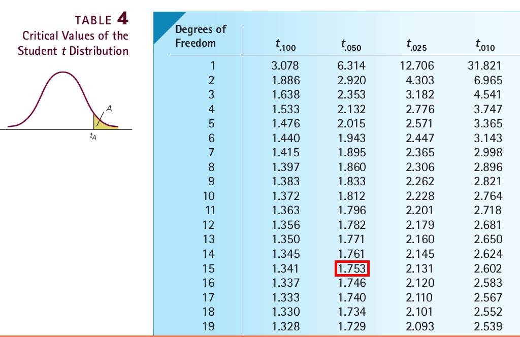
1.2.2 Student's t Distribution
- When the population standard deviation is unknown, for inference about the population mean, the (Student's) t distribution is used.
- Unlike the standard Normal distribution, there are many versions of t distribution, indexed by the so-called degrees of freedom.
- We use \(t_d\) to represent a random variable following the \(t\) distribution with \(d\) degrees of freedom.
- Use table 4 to find the number \(t_{\alpha, d}\) such that \(P(t_d > t_{\alpha, d}) = \alpha\).
For example, the number in the red box means \(P(t_{15} > 1.753) = 0.05\), so \(t_{0.05, 15} = 1.753\).
1.2.3 Confidence Interval
- When the population standard deviation of \(X\), denoted by \(\sigma\), is unknown, at Confidence Level \(1 - \alpha\), the confidence interval for the population mean \(\mu\) can be constructed as follows,
- Midpoint: \(\boxed{ \bar{X} }\);
- Critical Value: \(\boxed{ t_{\alpha/2, n-1} }\);
- Margin of Error: \(\boxed{ t_{\alpha/2, n-1} \cdot \frac{s}{\sqrt{n}} }\);
- Lower Confidence Limit (LCL): \(\boxed{ \bar{X} - t_{\alpha/2, n-1} \cdot \frac{s}{\sqrt{n}} }\);
- Upper Confidence Limit (UCL): \(\boxed{ \bar{X} + t_{\alpha/2, n-1} \cdot \frac{s}{\sqrt{n}} }\);
- Confidence Interval: \(\boxed{ \left[ \bar{X} - t_{\alpha/2, n-1} \cdot \frac{s}{\sqrt{n}}, \bar{X} + t_{\alpha/2, n-1} \cdot \frac{s}{\sqrt{n}} \right] }\);
- Width of Confidence Interval: \(\boxed{ 2 \cdot t_{\alpha/2, n-1} \cdot \frac{s}{\sqrt{n}} }\).
1.2.4 Hypothesis Testing
- When the population standard deviation of \(X\), denoted by \(\sigma\), is unknown, at Significance Level \(\alpha\),
- the t-test for \(\boxed{H_0: \mu \le \mu_0 \text{ vs } H_A: \mu > \mu_0}\) (which is equivalent to \(\boxed{H_0: \mu = \mu_0 \text{ vs } H_A: \mu > \mu_0}\)) can be constructed as follows,
- Test Statistic: \(\boxed{T = \frac{\sqrt{n}(\bar{X} - \mu_0)}{s}}\);
- Critical Value: \(\boxed{t_{\alpha, n-1}}\);
- Rejection Rule: Reject \(H_0\) if \(\boxed{T > t_{\alpha, n-1}}\).
- the t-test for \(\boxed{H_0: \mu \ge \mu_0 \text{ vs } H_A: \mu < \mu_0}\) (which is equivalent to \(\boxed{H_0: \mu = \mu_0 \text{ vs } H_A: \mu < \mu_0}\)) can be constructed as follows,
- Test Statistic: \(\boxed{T = \frac{\sqrt{n}(\bar{X} - \mu_0)}{s}}\);
- Critical Value: \(t_{1-\alpha, n-1}\), which equals \(\boxed{- t_{\alpha, n-1}}\)
- Rejection Rule: Reject \(H_0\) if \(T < t_{1-\alpha, n-1}\), which is equivalent to \(\boxed{T < - t_{\alpha, n-1}}\)
- the t-test for \(\boxed{H_0: \mu = \mu_0 \text{ vs } H_A: \mu \neq \mu_0}\) can be constructed as follows,
- Test Statistic: \(\boxed{T = \frac{\sqrt{n}(\bar{X} - \mu_0)}{s}}\);
- Critical Values: \(t_{1-\alpha/2, n-1}\) (which equals \(\boxed{- t_{\alpha/2, n-1}}\)) and \(\boxed{t_{\alpha/2, n-1}}\);
- Rejection Rule: Reject \(H_0\) if \(T > t_{\alpha/2, n-1}\) or \(T < - t_{\alpha/2, n-1}\), which is equivalent to \(\boxed{|T| > t_{\alpha/2, n-1}}\).
- the t-test for \(\boxed{H_0: \mu \le \mu_0 \text{ vs } H_A: \mu > \mu_0}\) (which is equivalent to \(\boxed{H_0: \mu = \mu_0 \text{ vs } H_A: \mu > \mu_0}\)) can be constructed as follows,
1.2.5 Example
- Suppose the students' scores follow a Normal distribution with unknown population mean \(\mu\) and unknown population standard deviation \(\sigma\).
- Q1: (Confidence Interval) If we randomly select \(16\) students and find their average score is \(79\) and sample standard deviation is \(3.5\), what is the confidence interval of the population mean at confidence level of \(90\%\)?
- Let \(X\) be the score of a student, then we know
- \(X\) follows a Normal distribution;
- the population mean of \(X\), denoted by \(\mu\), is unknown;
- the population standard deviation of \(X\), denoted by \(\sigma\), is unknown;
- the sample size \(n = 16\);
- the sample mean \(\bar{X} = 79\);
- the sample standard deviation \(s = 3.5\).
- To construct the confidence interval of \(\mu\) when \(\sigma\) is unknown,
- the confidence level is \(1 - \alpha = 90\%\), so \(\alpha = 0.1\);
- the midpoint of the confidence interval is \(\bar{X} = 79\);
- the critical value is \(t_{\alpha/2, n-1} = t_{0.1/2, 16-1} = t_{0.05, 15} = 1.753\);
- the margin of error is \(t_{\alpha/2, n-1} \cdot \frac{s}{\sqrt{n}} = 1.753 \cdot \frac{3.5}{\sqrt{16}} = 1.534\);
- the lower confidence limit is \(79 - 1.534 = 77.466\);
- the upper confidence limit is \(79 + 1.534 = 80.534\);
- the confidence interval is \([77.466, 80.534]\);
- the width of the confidence interval is \(2 \times 1.534 = 3.068\).
- Let \(X\) be the score of a student, then we know
- Q2: (Hypothesis Testing) If we randomly select \(16\) students and find their average score is \(79\) and sample standard deviation is \(3.5\), at \(5\%\) significance level, do we have sufficient evidence that the population mean is lower than \(80\)?
- Here we want to confirm the claim that \(\mu < 80\), so we let it be the alternative hypothesis. That is, we want to test \(H_0: \mu \ge 80\) vs \(H_A: \mu < 80\) (or equivalently \(H_0: \mu = 80\) vs \(H_A: \mu < 80\));
- The test statistic is \(T = \frac{\sqrt{n}(\bar{X} - \mu_0)}{s} = \frac{\sqrt{16}(79 - 80)}{3.5} = -1.143\);
- The significance level is \(\alpha = 5\%\);
- The critical value is \(- t_{\alpha, n-1} = - t_{0.05, 16-1} = - 1.753\);
- The rejection rule is: reject \(H_0\) if \(T < - t_{\alpha, n-1}\);
- Here \(T = -1.143 > -1.753 = -t_{\alpha, n-1}\), so we don't have enough evidence to reject \(H_0\) and thus don't have enough evidence to say that the population mean is lower than \(80\).
- Q3: (Hypothesis Testing) For Q3, at \(10\%\) significance level, do we have sufficient evidence that the population mean is lower than \(80\)?
- The hypotheses are the same, \(H_0: \mu \ge 80\) vs \(H_A: \mu < 80\) (or equivalently \(H_0: \mu = 80\) vs \(H_A: \mu < 80\));
- The test statistic is the same, \(T = \frac{\sqrt{n}(\bar{X} - \mu_0)}{s} = \frac{\sqrt{16}(79 - 80)}{3.5} = -1.143\);
- The significance level now is \(\alpha = 10\%\);
- The critical value now is \(-t_{\alpha, n-1} = -t_{0.1, 16-1} = - 1.341\);
- The rejection rule is the same: reject \(H_0\) if \(T < - t_{\alpha, n-1}\);
- Here \(T = -1.143 > -1.341 = -t_{\alpha, n-1}\), so we still don't have enough evidence to reject \(H_0\) and thus still don't have enough evidence to say that the population mean is lower than \(80\).
2 One-Population Inference: Population Variance
2.1 Assumptions and Notations
- \(X\): the random variable following a Normal distibution;
- \(\mu\): the (known or unknown) population mean of \(X\);
- \(\sigma^2\): the unknown population variance of \(X\);
- \(X_1, X_2, \dots, X_n\): the sample (observations) of \(X\);
- \(\bar{X}\): sample mean;
- \(s\): sample standard deviation.
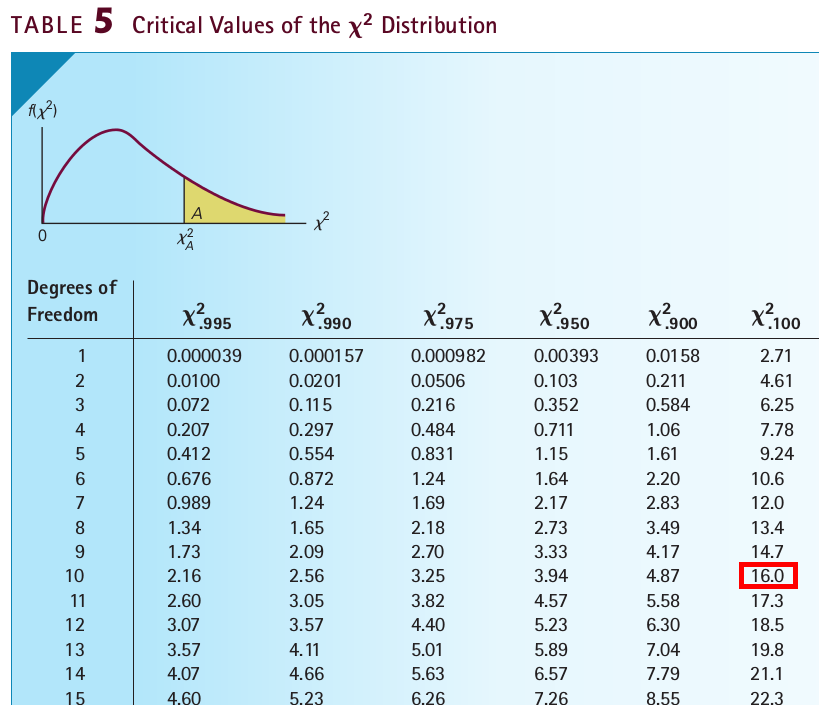
2.2 Student's \(\chi^2\) Distribution
- For inference about population variance, the \(\chi^2\) distribution is used.
- Unlike the standard Normal distribution, there are many versions of \(\chi^2\) distribution, indexed by the so-called degrees of freedom.
- We use \(\chi^2_d\) to represent a random variable following the \(\chi^2\) distribution with \(d\) degrees of freedom.
- Use table 5 to find the number \(\chi^2_{\alpha, d}\) such that \(P(\chi^2_d > \chi^2_{\alpha, d}) = \alpha\).
For example, the red box means \(P(\chi^2_{10} > 16) = 0.1\), so \(\chi^2_{0.1, 10} = 16\).
2.3 Confidence Interval
- The \(1-\alpha\) confidence interval of the unknown population variance \(\sigma^2\) is \[ \boxed{ \left[ \frac{(n-1)s^2}{\chi^2_{\alpha/2, n-1}}, \frac{(n-1)s^2}{\chi^2_{1 - \alpha/2, n-1}} \right] } \]
- \(\frac{(n-1)s^2}{\chi^2_{\alpha/2, n-1}}\) is called the Lower Confidence Level;
- \(\chi^2_{\alpha/2, n-1}\) is called the Critical Value for Lower Confidence Level.
- \(\frac{(n-1)s^2}{\chi^2_{1 - \alpha/2, n-1}}\) is called the Upper Confidence Level;
- \(\chi^2_{1- \alpha/2, n-1}\) is called the Critical Value for Upper Confidence Level.
2.4 Hypothesis Testing
- At Significance Level \(\alpha\),
- the test for \(\boxed{ H_0: \sigma^2 \le \sigma_0^2 \text{ vs } H_A: \sigma^2 > \sigma_0^2 }\) (which is equivalent to \(\boxed{ H_0: \sigma^2 = \sigma_0^2 \text{ vs } H_A: \sigma^2 > \sigma_0^2 }\)) can be constructed as follows,
- Test Statistic: \(\boxed{ T = \frac{(n-1)s^2}{\sigma_0^2} }\);
- Critical Value: \(\boxed{ \chi^2_{\alpha, n-1} }\);
- Rejection Rule: Reject \(H_0\) if \(\boxed{ T > \chi^2_{\alpha, n-1} }\).
- the test for \(\boxed{ H_0: \sigma^2 \ge \sigma_0^2 \text{ vs } H_A: \sigma^2 < \sigma_0^2 }\) (which is equivalent to \(\boxed{ H_0: \sigma^2 = \sigma_0^2 \text{ vs } H_A: \sigma^2 < \sigma_0^2 }\)) can be constructed as follows,
- Test Statistic: \(\boxed{ T = \frac{(n-1)s^2}{\sigma_0^2} }\);
- Critical Value: \(\boxed{ \chi^2_{1 - \alpha, n-1} }\);
- Rejection Rule: Reject \(H_0\) if \(\boxed{ T < \chi^2_{1 - \alpha, n-1} }\).
- the test for \(\boxed{ H_0: \sigma^2 = \sigma_0^2 \text{ vs } H_A: \sigma^2 \neq \sigma_0^2 }\) can be constructed as follows,
- Test Statistic: \(\boxed{ T = \frac{(n-1)s^2}{\sigma_0^2} }\);
- Critical Values: \(\boxed{ \chi^2_{1 - \alpha/2, n-1} } \text{ and } \boxed{ \chi^2_{\alpha/2, n-1} }\);
- Rejection Rule: Reject \(H_0\) if \(\boxed{ T > \chi^2_{\alpha/2, n-1} \text{ or } T < \chi^2_{1 - \alpha/2, n-1} }\).
- the test for \(\boxed{ H_0: \sigma^2 \le \sigma_0^2 \text{ vs } H_A: \sigma^2 > \sigma_0^2 }\) (which is equivalent to \(\boxed{ H_0: \sigma^2 = \sigma_0^2 \text{ vs } H_A: \sigma^2 > \sigma_0^2 }\)) can be constructed as follows,
2.5 Example
- Suppose the students' scores follow a Normal distribution with unknown population mean \(\mu\) and unknown population variance \(\sigma^2\).
- Q1: (Confidence Interval) If we randomly select \(16\) students and find their average score is \(79\) and sample standard deviation is \(3.5\), what is the confidence interval of the population variance at confidence level of \(90\%\)?
- Let \(X\) be the score of a student, then we know
- \(X\) follows a Normal distribution;
- the population variance of \(X\), denoted by \(\sigma^2\), is unknown;
- the sample size \(n = 16\);
- the sample mean \(\bar{X} = 79\);
- the sample standard deviation \(s = 3.5\) and thus the sample variance is \(s^2 = 3.5^2 = 12.25\).
- To construct the confidence interval of the unknown \(\sigma^2\),
- the confidence level is \(1 - \alpha = 90\%\), so \(\alpha = 0.1\);
- the critical values are
- \(\chi^2_{1 - \alpha/2, n-1} = \chi^2_{1 - 0.1/2, 16-1} = \chi^2_{0.95, 15} = 7.26\);
- \(\chi^2_{\alpha/2, n-1} = \chi^2_{0.1/2, 16-1} = \chi^2_{0.05, 15} = 25.0\);
- the confidence interval is \(\left[ \frac{(n-1)s^2}{\chi^2_{\alpha/2, n-1}}, \frac{(n-1)s^2}{\chi^2_{1 - \alpha/2, n-1}} \right]\) \(=\) \(\left[ \frac{(16-1)\cdot 3.5^2}{25}, \frac{(16-1)\cdot 3.5^2}{7.26} \right]\) \(=\) \([7.35, 25.31]\)
- the width of the confidence interval is \(25.31 - 7.35 = 17.96\).
- Let \(X\) be the score of a student, then we know
- Q2: (Hypothesis Testing) If we randomly select \(16\) students and find their average score is \(79\) and sample standard deviation is \(3.5\), at \(5\%\) significance level, do we have sufficient evidence that the population variance is lower than \(13\)?
- Here we want to confirm the claim that \(\sigma^2 < 13\), so we let it be the alternative hypothesis. That is, we want to test \(H_0: \sigma^2 \ge 13\) vs \(H_A: \sigma^2 < 13\) (or equivalently \(H_0: \sigma^2 = 13\) vs \(H_A: \sigma^2 < 13\)) where \(\sigma_0^2 = 13\);
- The test statistic is \(T = \frac{(n-1)s^2}{\sigma_0^2} = \frac{(16-1)\cdot 3.5^2}{13} = 14.135\);
- The significance level is \(\alpha = 5\%\);
- The critical value is \(\chi^2_{1-\alpha, n-1} = \chi^2_{1-0.05, 16-1} = 7.26\);
- The rejection rule is: reject \(H_0\) if \(T < \chi^2_{1-\alpha, n-1}\);
- Here \(T = 14.135 > 7.26 = \chi^2_{\alpha, n-1}\), so we don't have enough evidence to reject \(H_0\) and thus don't have enough evidence to say that the population variance is lower than \(13\).
3 One-Population Inference: Population Proportion
3.1 Notations
- \(p\): the unknown population proportion (probability) of the event of interest.
- \(\hat{p}\): the sample proportion (relative frequency) of the event among the \(n\) independent trials.
3.2 Sampling Distribution
- Suppose \(X \sim Binomial(n, p)\). When \(np\) and \(n(1−p)\) are greater than or equal to \(5\), \(\hat{p}\) is approximately Normally distributed with
- population mean \(\boxed{ \mu_{\hat{p}} = E(\hat{p}) = p }\);
- population variance \(\boxed{ \sigma_{\hat{p}}^2 = Var(\hat{p}) = \frac{p(1-p)}{n} }\).
- That is, \[ \boxed{ \hat{p} \sim N \left( p, \frac{p(1-p)}{n} \right) } \]
3.3 Confidence Interval
3.3.1 Construction
- At Confidence Level \(1 - \alpha\), the confidence interval for the unknown population proportion \(p\) is constructed as follows,
- Midpoint: \(\boxed{ \hat{p} }\);
- Critical Value: \(\boxed{ Z_{\alpha/2} }\);
- Margin of Error: \(\boxed{ Z_{\alpha/2} \cdot \sqrt{\frac{\hat{p}(1-\hat{p})}{n}} }\);
- Lower Confidence Limit (LCL): \(\boxed{ \hat{p} - Z_{\alpha/2} \cdot \sqrt{\frac{\hat{p}(1-\hat{p})}{n}} }\);
- Upper Confidence Limit (UCL): \(\boxed{ \hat{p} + Z_{\alpha/2} \cdot \sqrt{\frac{\hat{p}(1-\hat{p})}{n}} }\);
- Confidence Interval: \(\boxed{ \left[ \hat{p} - Z_{\alpha/2} \cdot \sqrt{\frac{\hat{p}(1-\hat{p})}{n}}, \hat{p} + Z_{\alpha/2} \cdot \sqrt{\frac{\hat{p}(1-\hat{p})}{n}} \right] }\);
- Width of Confidence Interval: \(\boxed{ 2 \cdot Z_{\alpha/2} \cdot \sqrt{\frac{\hat{p}(1-\hat{p})}{n}} }\);
3.3.2 Sample Size
At confidence level \(1-\alpha\), to achieve a confidence interval for the population proportion \(p\) whose margin of error is no wider than \(M\), the smallest sample size needed is \[ \boxed{ n = \left( \frac{Z_{\alpha/2}}{2M} \right)^2 } \]
If the value of \(n\) calculated by the formula is not an integer, then we should round it up in order to ensure the actual margin of error is no wider than \(M\).
3.4 Hypothesis Testing
- At Significance Level \(\alpha\),
- the test for \(\boxed{ H_0: p \le p_0 \text{ vs } H_A: p > p_0 }\) (which is equivalent to \(\boxed{ H_0: p = p_0 \text{ vs } H_A: p > p_0 }\)) can be constructed as follows,
- Test Statistic: \(\boxed{ T = \frac{\hat{p} - p_0}{\sqrt{\frac{p_0 (1-p_0)}{n}}} }\);
- Critical Value: \(\boxed{ Z_{\alpha} }\);
- Rejection Rule: Reject \(H_0\) if \(\boxed{ T > Z_{\alpha} }\).
- the test for \(\boxed{ H_0: p \ge p_0 \text{ vs } H_A: p < p_0 }\) (which is equivalent to \(\boxed{ H_0: p = p_0 \text{ vs } H_A: p < p_0 }\)) can be constructed as follows,
- Test Statistic: \(\boxed{ T = \frac{\hat{p} - p_0}{\sqrt{\frac{p_0 (1-p_0)}{n}}} }\);
- Critical Value: \(Z_{1-\alpha}\), which equals \(\boxed{ -Z_{\alpha} }\);
- Rejection Rule: Reject \(H_0\) if \(\boxed{ T < -Z_{\alpha} }\).
- the test for \(\boxed{ H_0: p = p_0 \text{ vs } H_A: p \neq p_0 }\) can be constructed as follows,
- Test Statistic: \(\boxed{ T = \frac{\hat{p} - p_0}{\sqrt{\frac{p_0 (1-p_0)}{n}}} }\);
- Critical Value: \(Z_{1-\alpha/2}\) (which equals \(\boxed{ -Z_{\alpha/2} }\)) and \(\boxed{ Z_{\alpha/2} }\);
- Rejection Rule: Reject \(H_0\) if \(\boxed{ |T| > Z_{\alpha/2} }\) (ie, \(T > Z_{\alpha/2}\) or \(T < Z_{1-\alpha/2}\)).
- the test for \(\boxed{ H_0: p \le p_0 \text{ vs } H_A: p > p_0 }\) (which is equivalent to \(\boxed{ H_0: p = p_0 \text{ vs } H_A: p > p_0 }\)) can be constructed as follows,
3.5 Example
- Suppose the proportion of female students in the university is \(p\).
- Q1: (Confidence Interval) If we randomly select \(100\) students and find \(45\) of them are female, what is the confidence interval for the population proportion of female students, \(p\), at confidence level of \(90\%\)?
- We know the sample proportion of female students \(\hat{p} = \frac{45}{100} = 0.45\), and want to construct the \(90\%\) confidence interval for the population proportion \(p\).
- To construct the confidence interval of the unknown population proportion \(p\),
- the confidence level is \(1−\alpha = 90\%\), so \(\alpha=0.1\);
- the midpoint is \(\hat{p} = 0.45\);
- the critical value is \(Z_{\alpha/2} = Z_{0.05} = 1.64\);
- the margin of error is \(Z_{\alpha/2} \sqrt{\frac{\hat{p}(1-\hat{p})}{n}} = 1.64 \sqrt{\frac{0.45(1-0.45)}{100}} = 0.0816\);
- the lower confidence limit is \(0.45 - 0.0816 = 0.3684\);
- the upper confidence limit is \(0.45 + 0.0816 = 0.5316\);
- the confidence interval is \([0.3684, 0.5316]\)
- the width of the confidence interval is \(2 \cdot 0.0816 = 0.1632\).
- Q2: (Sample Size) At confidence level \(90\%\), to achieve a confidence interval no wider than \(10\%\), what is the smallest sample size needed?
- the confidence level is \(1 - \alpha = 90\%\), so \(\alpha = 0.1\);
- the critical value is \(Z_{\alpha/2} = Z_{0.1/2} = Z_{0.05} = 1.64\);
- since the width of the confidence interval is \(2M\) where \(M\) is the margin of error, to let \(2M < 10\% = 0.1\), we need \(M < 0.05\);
- by formula, to achieve \(M<0.05\), the smallest sample size should be \(n = \left( \frac{z_{\alpha/2}}{2M} \right)^2 = \left( \frac{1.64}{2\cdot 0.05} \right)^2 = 268.96 \approx 269\).
- Q3: (Hypothesis Testing) If we randomly select \(100\) students and find \(45\) of them are female, at \(5\%\) significance level, do we have sufficient evidence that the population proportion of female is lower than \(50\%\)?
- Here we want to confirm the claim that \(p<0.5\), so we let it be the alternative hypothesis. That is, we want to test \(H_0: p \ge 0.5\) vs \(H_A: p < 0.5\) (or equivalently \(H_0: p = 0.5\) vs \(H_A: p < 0.5\)) where \(p_0 = 0.5\) and \(n=100\);
- The test statistic is \(T = \frac{\hat{p} - p_0}{\sqrt{\frac{p_0 (1-p_0)}{n}}} = \frac{0.45 - 0.5}{\sqrt{\frac{0.5 (1-0.5)}{100}}} = -1\);
- The significance level is \(\alpha = 5\%\);
- The critical value is \(−Z_{\alpha} = −Z_{0.05} = −1.64\);
- The rejection rule is: reject \(H_0\) if \(T < −Z_{\alpha}\);
- Here \(T = −1 > −1.64 = −Z_{\alpha}\), so we don't have enough evidence to reject \(H_0\) and thus don't have enough evidence to say that the population proportion of female is lower than \(50\%\).
4 References
- Keller, Gerald. (2015). Statistics for Management and Economics, 10th Edition. Stamford: Cengage Learning.