STAT 3360 Notes
Table of Contents
- 1. STAT 3360.001 Notes
- 2. Basics
- 3. Graphical Description: Nominal Data
- 4. Graphical Description: Ordinal Data
- 5. Graphical Description: Interval Data
- 6. Numerical Description: Interval Data
- 7. References
1 STAT 3360.001 Notes
- This notes covers all materials discussed in the lecture sessions of STAT 3360.001, 2016 Spring.
- This notes covers not only the materials discussed in the lecture sessions, but also some other important notions, explanations and comments. To do the homework or prepare for the quizzes and exams, you may focus just on the topics discussed in class. However, it is strongly recommended that you read through the whole notes in order to view a bigger picture of statistics.
- This notes is a supplement to the lecture sessions, NOT a substitute for it. Without regular attendance in the lecture sessions, you may find it hard to understand the materials in this notes. Actually, the aim of this notes is to save your time for copying blackboard notes and to provide a convenient reference outside the classroom.
- The organization of this notes may be different from that of the textbook or the syllabus outline.
- All data used in this notes are fake, not real.
- This notes is subject to modification and correction without notifications. The lower-left corner of this webpage shows the time of last update.
- Suggestions, corrections and critiques are sincerely welcomed.
2 Basics
2.1 Population
- A population is the group of all items of interest.
- For example,
- all students at UTD constitute a population,
- all beverages sold at Walwart constitute a population.
2.2 Sample
- A sample is a subset of the studied population.
- For example,
- "all students in STAT 3360" is a sample from the population "all UTD students",
- "all male students at UTD" is a sample from the poputation "all UTD students",
- "all students at UTD taller than 67 inches" is a sample from the poputation "all UTD students",
- "all students at UTD heavier than 120 pounds" is a sample from the poputation "all UTD students",
- "all students at UTD getting B or above for STAT 3360" is a sample from the poputation "all UTD students",
- "all juice sold at Walmart" is a sample from the population "all beverages sold at Walmart",
- "all beverages sold at Walmart more expensive than $2" is a sample from the population "all beverages sold at Walmart".
2.3 Variable
- A variable is some characteristic of a population or sample.
- For example,
- the course a UTD student takes in Monday afternoon is a variable,
- the gender of a UTD student is a variable,
- the height of a UTD student is a variable,
- the weight of a UTD student is a variable,
- the STAT 3360 grade of a UTD student is a variable,
- the type of a beverage sold at Walmart is a variable,
- the price of a beverage sold at Walmart is a variable.
2.4 Values
- The values of the variable are the possible observations of the variable.
- For example,
- the values of the variable the course a UTD student takes in Monday afternoon are STAT 3360, MATH 1326, MATH 2413, …,
- the values of the variable the gender of a UTD student are male, female,
- the values of the variable the height of a UTD student are all numbers greater than \(0\) (theoretically),
- the values of the variable the weight of a UTD student are all numbers greater than \(0\) (theoretically),
- the values of the variable the STAT 3360 grade of a UTD student are A, B, C, D, F,
- the values of the variable the type of a beverage sold at Walmart are soda, juice, water, alcohol, other,
- the values of the variable the price of a beverage sold at Walmart are all numbers greater than \(0\) (theoretically).
2.5 Data
- Data are the observed values of a variable.
- For example,
- if in Monday afternoon at UTD Alicia and Bill take STAT 3360 and Chris takes MATH 2413, then the data of the variable the course a UTD student takes in Monday afternoon are STAT 3360, STAT 3360, MATH 2413,
- if UTD student David is a male, Emily is a female, Frank is a male, Gabe is a male, then the data of the variable the gender of a UTD student are Male, Female, Male, Male,
- if UTD student Henry is \(68\) inches in height, Ivan is \(69\) inches, Jeremy is \(67\) inches and Katy is \(67\) inches, then the data of the variable the height of a UTD student are \(68, 69, 67, 67\) with inches as the unit,
- if Lisa gets B and Mike gets C for STAT 3360, then the data of the variable the STAT 3360 grade of a UTD student are B, C,
- if Nicholas bought both soda and water and Olivia bought water from Walmart, then the data of the variable the type of a beverage sold at Walmart are soda, water, water
2.6 Type of Variable/Data
2.6.1 Interval Variable/Data
- Definition
- Also known as quantitative or numerical variable/data.
- Values are real numbers.
- All calculations are valid.
- Data may be treated as ordinal or nominal.
- Example
- The values of the variable height of a UTD student are positive real numbers, so it is an interval variable.
- The values of the variable weight of a UTD student are positive real numbers, so it is an interval variable.
2.6.2 Ordinal Variable/Data
- Definition
- Values are just symbols even if coded by numbers.
- Values must represent the ranked order of the data.
- Calculations based on an ordering process are valid.
- Data may be treated as nominal but not as interval.
- Based on the context, sometimes ordinal variables/data are also classified as categorial variable/data.
- Example
- The values of the variable STAT 3360 grade of a UTD student are non-numerical (A, B, C, D, F) and there is an order between them, so it is an ordinal variable.
- Even if we use "1", "2", "3", "4", "5" to represent A, B, C, D, F respectively, the variable STAT 3360 grade of a UTD student is still ordinal, not numerical. "1", "2", "3", "4" and "5" are just symbols like A, B, C, D, F, not real numbers for which arithmetic operations are meaningful.
2.6.3 Nominal Variable/Data
- Definition
- Also known as qualitative or categorial variable/data.
- Values are just symbols even if coded by numbers.
- Values are the arbitrary numbers that represent categories.
- Only calculations based on the frequencies or percentages of occurrence are valid.
- Data may not be treated as ordinal or interval.
- Example
- The values of the variable gender of a UTD student are non-numerical and there is no order between them, so it is an nominal variable.
- Even if we use "1" and "2" to represent Male and Female respectively, the variable gender of a UTD student is still nominal, not numerical. "1" and "2" are just symbols like Male and Female or M and F, not real numbers for which arithmetic operations are meaningful.
2.6.4 Hierarchy between Types
- Interval variables/data can be treated as ordinal ones.
For example, we may convert the interval variable "height" into an ordinal variable "height class", the values which are short (if height < 55 inches), medium (if 55 inches < height < 65 inches), tall (if height > 65 inches). Note there is an order between the values short, medium, tall.
- Orodinal variable/data can be treated as nominal ones.
For example, we may convert the ordinal variable "height class" to a nominal variable "medium height or not", the values of which are YES (if height class = medium), NO (if height class = short or tall). Note that there is no order between the values YES and NO: some people in the NO class are taller than the people in the YES class, while some people in the NO class are shorter than the people in the YES class.
- Nominal variables/data can not be treated as ordinal ones, and ordinal variables/data can not be treated as numerical ones.
Suppose we get a data which uses number (symbol) \(1\) to represent short, \(2\) for medium and \(3\) for tall. Then we can't convert \(1, 2, 3\) into numerical values: we can't say a tall person is \(3\) inches in height, and we don't know what numercial height value exactly corresponds to the symbol "\(3\)".
- To summarize, the conversion between the three types of variables/data is
\[ Interval \overset{\checkmark}{\underset{\times}\rightleftharpoons} Ordinal \overset{\checkmark}{\underset{\times}\rightleftharpoons} Nominal \]
2.6.5 Why Do We Care About the Type
- For different types of variables/data, we have different statistical techniques. This is the main reason why we need pay attention to the type of variable/data before any statistical analysis.
3 Graphical Description: Nominal Data
3.1 Raw Data: Student Section and Gender
Suppose we have the follwing information of 51 students in STAT 3360.
StudentID Section Gender StudentID Section Gender StudentID Section Gender 1 SEC3 Male 18 SEC3 Male 35 SEC3 Female 2 SEC1 Male 19 SEC1 Male 36 SEC2 Male 3 SEC3 Male 20 SEC2 Female 37 SEC3 Male 4 SEC1 Female 21 SEC3 Male 38 SEC2 Female 5 SEC1 Male 22 SEC1 Female 39 SEC2 Female 6 SEC1 Male 23 SEC1 Female 40 SEC3 Male 7 SEC3 Male 24 SEC1 Male 41 SEC2 Female 8 SEC3 Female 25 SEC3 Female 42 SEC1 Female 9 SEC3 Female 26 SEC3 Female 43 SEC1 Female 10 SEC2 Male 27 SEC2 Male 44 SEC1 Female 11 SEC3 Male 28 SEC3 Female 45 SEC3 Female 12 SEC1 Female 29 SEC3 Male 46 SEC1 Male 13 SEC1 Female 30 SEC2 Female 47 SEC3 Female 14 SEC2 Female 31 SEC1 Female 48 SEC2 Male 15 SEC2 Female 32 SEC2 Male 49 SEC3 Female 16 SEC3 Male 33 SEC2 Female 50 SEC3 Male 17 SEC3 Female 34 SEC2 Female 51 SEC3 Male - Question: what can you learn from the raw data?
- It seems quite hard for us to get useful information from the raw data at the first glance, especially when the number of observations is huge. Therefore, we need some quick summary of the data.
- To quickly summarize and display the information inside the data, we
- first calculate the quantities of summary, and then
- use tabular and graphical techniques to display these quantities of summary.
3.2 Frequency
- The Frequency of a value of the variable is the count of that value in the sample.
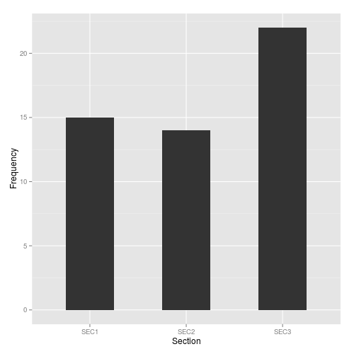
- For the variable Section, the frequencies of SEC1, SEC2 and SEC3 are \(15\), \(14\) and \(22\), respectively.
3.3 Relative Frequency
- The Relative Frequency of a value of the variable is the proportion of that value in the sample, that is \[ \boxed{\text{relative frequency of the value} = \frac{\text{frequency of the value}}{\text{total count of all values of the variable}}} \]
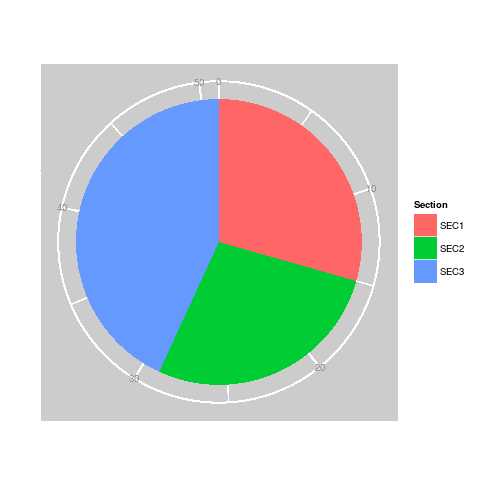
- For the variable Section, the relative frequencies of SEC1, SEC2 and SEC3 are \(15/51 = 29.41\%\), \(14/51=27.45\%\) and \(22/51=43.14\%\), respectively.
3.4 One-Variable Table: Frequency Table
- Each column corresponds to a value of the variable.
- Each cell in the first row indicates the frequency of the corresponding value.
- Each cell in the second row indicates the relative frequency of the corresponding value.
- The last column is Total
For the variable Section, the frequency and relative frequency table is as follows
Section SEC1 SEC2 SEC3 Total Frequency (Count) 15 14 22 51 Relative Frequency (Proportion) \(29.41\%\) \(27.45\%\) \(43.14\%\) \(100\%\)
3.5 One-Variable Graph: Bar Chart
- x-axis contains the values of the nominal variable.
- y-axis indicates the frequency of each value by a vertical bar;
- bars
- All the bars should have the same width, while the width itself is arbitrary;
- The bars don't have to be adjacent;
- The order between the bars doesn't matter for nominal data.
For the variable Section, the frequency bar chart is
3.6 One-Variable Graph: Pie Chart
- Starting from 12 o'clock, draw the slices or the pie consecutively in the clockwise direction;
- \[ \boxed{ \text{The degree of each slice = the relative frequency} \times 360^{\circ} } \]
- We can (not required though) draw the slices in the descending order of their degrees, which makes the chart even more informative.
For the variable Section, the bar chart is
3.7 Two-Variable Table: Cross-Classification
- A two-dimensional table;
- Each column corresponds to a value of the 1st variable;
- Each row corresponds to a value of the 2nd variable;
- Each cell in the table indicates the frequency or relative frequency corresponding to the current combination of the values of the two variables.
For the data Student Section and Gender, if we consider variables Section and Gender at the same time, then the cross-classification table is
Table Female Male Row Total SEC1 9 6 15 SEC2 9 5 14 SEC3 10 12 22 Column Total 28 23 51 or in the other way
SEC1 SEC2 SEC3 Row Total Female 9 9 10 28 Male 6 5 12 23 Column Total 15 14 22 51
4 Graphical Description: Ordinal Data
- The graphical descriptive techniques for ordinal data are the same as those for nominal data, except for one special requirement: for ordinal data, the order (either ascending or descending) between the values of the variable should be kept when we make the frequency table, bar chart and pie chart.
5 Graphical Description: Interval Data
5.1 Raw Data: Student Weight and Height
Suppose we have the following information of 51 students in STAT 3360.
- To save space in the webpage, the whole data is split into three blocks with each block having 17 observations, and the three blocks are put one by one horizontally from left to right.
- Within each block, every row stands for an individual student: student ID is a symbol (not a numerical number by nature!) for identifying this student, Height is the height of this student and Weight is the weight of this student.
- For simplicity, observations are rounded to integers, but all notions and techniques introduced in this section can be applied to non-integers in exactly the same way.
StudentID Height Weight StudentID Height Weight StudentID Height Weight 1 66 113 18 66 130 35 72 140 2 72 136 19 69 143 36 69 129 3 69 153 20 71 138 37 67 142 4 68 142 21 67 124 38 68 121 5 68 144 22 68 141 39 68 131 6 69 123 23 69 144 40 64 107 7 70 141 24 63 98 41 69 124 8 70 136 25 68 130 42 65 125 9 68 112 26 68 142 43 70 140 10 67 121 27 67 130 44 68 137 11 66 127 28 71 142 45 66 106 12 68 114 29 67 132 46 69 129 13 68 126 30 67 108 47 67 146 14 67 122 31 65 114 48 68 117 15 68 116 32 70 103 49 70 144 16 71 140 33 66 121 50 69 135 17 66 130 34 68 126 51 70 147 - Just as we did for nominal and ordinal data, we use tabular and graphical techniques to display the summary of the information in the data.
5.2 One-Variable Graph: Stem-and-Leaf Plot
- A stem-and-leaf plot puts all the raw data together in a concise way, which also shows the frequency of each stem.
- For integer-valued interval data, to draw the stem-and-leaf plot
- split each observation into two stem and leaf
- use the last digit(single digit) as the leaf,
- use the other digits as the stem,
- find all different values of the stem over the whole data, and list them vertically on the left, in an ascending order,
- for each stem, find all corrsponding leafs over the whole data, and list them horizontally to the right of the stem, in an ascending order.
- split each observation into two stem and leaf
- What about non-integer-valued data? Well, we don't consider it in this course. Actually, the idea is the same: to cut the number into stem and leaf at some place. One may
- either round the demical observations to integers and then use the stem-and-plot for integers,
- or use the decimal point as the splitting delimitor if there is only one decimial digit in all the observations,
- or let all observations have the same number of decimal digits (by rounding or padding), and then use the last digit as the leaf and all digits before it as the stem.
- For the variable Weight,
- In the raw data
- The 1st observation of Weight is \(113\), so we split is as \(11|3\) where \(11\) is the stem and \(3\) is the leaf
- The 2nd observation of Weight is \(136\), so we split is as \(13|6\) where \(13\) is the stem and \(6\) is the leaf
- \(\dots\)
- The 24th observation of Weight is \(98\), so we split is as \(9|8\) where \(9\) is the stem and \(8\) is the leaf
- \(\dots\)
- The 51th observation of Weight is \(147\), so we split is as \(14|7\) where \(14\) is the stem and \(7\) is the leaf
The stem-and-leaf plot is
stem | leaf
   9 | 8
  10 | 3678
  11 | 234467
  12 | 1112344566799
  13 | 00012566678
  14 | 000112222344467
  15 | 3
- In the stem-and-leaf plot
- The left-hand side of the vertical line includes all different values of the stem, \(9, 10, 11, 12, 13, 14, 15\).
- The values of stems are listed vertically in an ascending order.
- In the first row of the plot, \(9 | 8\) means there is only one number in the raw data whose stem is \(9\) and leaf is \(8\). That is to say, \(98\) is the only number in the raw data beginning with \(9\).
- \(10 | 3678\) mean there are four numbers in the raw data whose stems are \(10\) and leaves are \(3, 6, 7\) and \(8\). That is to say, \(103, 106, 107\) and \(108\) are the only four numbers in the raw data beginning with \(10\).
- The same for the other rows.
- For each stem, the leaves are listed horizontally in an ascending order.
- In the raw data
5.3 One-Variable Table
- Similar to the table of frequencies and relative frequencies for categorical (nominal, ordinal) data.
- Unlike categorical data, for interval data, there are no pre-defined classes so that we have to construct the classes first (eg, the number of classes and the scope of each class) before we can get the count for each class. Fortunately, construction of classes is not required by this course and the classes will be given by the problem.
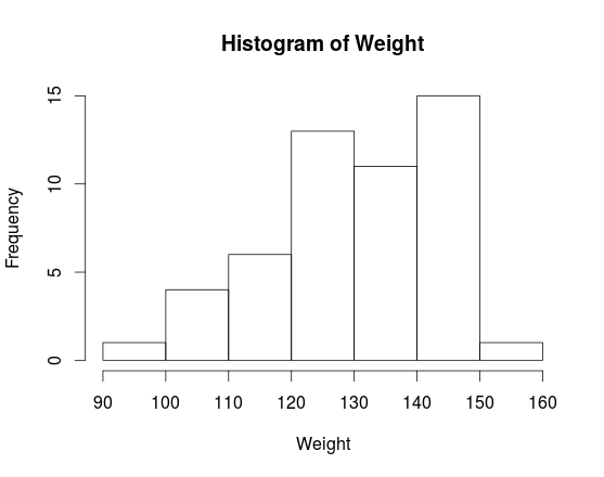
For the variable Weight, if we separate its values into \([90, 100), [100, 110), [110, 120), [120, 130), [130, 140), [140, 150)\) and \([150, 160)\), then we have the following frequency and relative frequency table
Weight [90, 100) [100, 110) [110, 120) [120, 130) [130, 140) [140, 150) [150, 160) Total Frequency (Count) 1 4 6 13 11 15 1 51 Relative Frequency (Proportion) \(1.96\%\) \(7.84\%\) \(11.76\%\) \(31.37\%\) \(25.49\%\) \(21.57\%\) \(1.96\%\) \(100\%\)
5.4 One-Variable Graph: Histogram
5.4.1 Introduction
- For categorical data, we use bar charts to display the frequencies. Similarly, for interval data, once the classes are constructed and the frequencies of classes are obtain, we can make a bar-chart-like graph, called histogram.
5.4.2 Components of Histograms
- x-axis contains the classes of the values of the data
- y-axis indicates the frequency of class, indicated by a vertical bar;
- bars
- All the bars should have the same width, because the intervals of classes have the same length.
- The bars have to be adjacent;
- The order between the bars matters because the there is an order between the classes.
5.4.3 Histogram and Bar Chart
- Bar charts are used for nominal or ordinal data, while histograms are used for interval data.
- The x-axis of a bar chart contains the categorical values of the variable, while the x-axis of a histogram is the real number line which includes all possble numerical values of the variable.
- The bars of a bar chart can be separate, while the bars of a histogram have to be adjacent.
- For nominal data, since there is no specific order between different values of the variable, the order of the bars is arbitrary. For numeric data, since there is a strict order on the real number line, the order between the bars is fixed.
5.4.4 How to Draw the Histogram
- Clearly, first of all, we should separate the values of the data into several classes and get the frequency and relative frequency of each group. Now the questions are : how do we determine the number of class?
- The answer sounds good : in this course, every time you are asked to draw a histogram, the classes will be given so that you don't have to construct them by yourself.
5.4.5 Example
For the above given classes of variable Weight, we already have the frequency and relative frequency table, so the histogram can be drawn as follows.
6 Numerical Description: Interval Data
6.1 Raw Data: Student Weight and Height
For convenience, let's use just the first 12 observations in the Student Weight and Height data. For simplicity, observations are rounded to integers, but all notions and techniques introduced in this section can be applied to non-integers in exactly the same way.
StudentID Height Weight 1 66 113 2 72 136 3 69 153 4 68 142 5 68 144 6 69 123 7 70 141 8 70 136 9 68 112 10 67 121 11 66 127 12 68 114
6.2 Introduction
- Base on the raw data, we are interested in at least the following questions
- What are the medium height and medium weight of the students? That is, we need a measure of central location.
- Do all students have similar height and weight? That is, we need a measure of variability.
- How many values are below a specific threshold? That is, we need a measure of relative standing.
- What is the relationship between height and weight? (For example, we tend to believe taller people are also heavier.) That is, we need a measure of relationship.
6.3 Measures of Central Location
6.3.1 Sample Mean
- Suppose we have a sample consisting of \(n\) observations \(x_1, x_2, \dots, x_n\). Then the sample mean \(\bar{x}\) is defined as the average of all observations, that is, \[ \boxed {\bar{x} = \frac{\sum\limits_{i=1}^{n} x_i}{n}} \]
- For the Student Weight and Height data
- the sample size is \(n=12\)
- the sample mean of Height is \(\frac{66+72+69+\cdots+68}{51} = 68.42\).
- the sample mean of Weight is \(\frac{113+136+153+\cdots+114}{51} = 130.17\).
6.3.2 Sample Median
- Intuitively, the sample median is the number "in the middle place". For example,
- if we have five numbers \(2, 3, 5, 8, 10\), then \(5\) is the "middle place" and called the sample median because \(2\) and \(3\) are less than it and \(8\) and \(10\) are greater than it.
- if we have six numbers \(2, 3, 5, 8, 10, 21\), then both \(5\) and \(8\) are in the "middle place". In this case, we call the average of \(5\) and \(8\) (ie, \(\frac{5+8}{2} = 6.5\)) the sample median.
- Here is the formal formula for calculating the sample median.
- Suppose we have a sample consisting of \(n\) observations \(x_1, x_2, \dots, x_n\).
- Let \(x_{(1)}, x_{(2)}, \dots, x_{(n)}\) be the ordered data, from smallest to largest.
- Then the sample median \(M\) is defined as
- the value of \( x_{\left( \frac{n+1}{2} \right)} \), if \(n\) is odd;
- the average value of \( x_{\left( \frac{n}{2} \right)} \) and \( x_{\left( \frac{n}{2} + 1 \right)} \), if \(n\) is even.
- For the Student Weight and Height data,
the ordered values of Height are
\(x_{(1)}\) \(x_{(2)}\) \(x_{(3)}\) \(x_{(4)}\) \(x_{(5)}\) \(x_{(6)}\) \(x_{(7)}\) \(x_{(8)}\) \(x_{(9)}\) \(x_{(10)}\) \(x_{(11)}\) \(x_{(12)}\) 66 66 67 68 68 68 68 69 69 70 70 72 - since the sample size is \(n=12\), which is an even number, the sample median is the average value of \(x_{(\frac{12}{2})} = x_{(6)}\) and \(x_{(\frac{12}{2}+1)} = x_{(7)}\), which is \(\frac{68+68}{2} = 68\).
- Suppose now we remove the last observation of Height, and regards the remaining \(11\) observations (66, 72, 69, 68, 68, 69, 70, 70, 68, 67, 66) as our new data. Then
the ordered values of Height are
\(x_{(1)}\) \(x_{(2)}\) \(x_{(3)}\) \(x_{(4)}\) \(x_{(5)}\) \(x_{(6)}\) \(x_{(7)}\) \(x_{(8)}\) \(x_{(9)}\) \(x_{(10)}\) \(x_{(11)}\) 66 66 67 68 68 68 69 69 70 70 72 - since the sanple size of the new data is \(n=11\), which is an odd number, the sample median is just \(x_{(\frac{11+1}{2})} = x_{6} = 68\).
6.3.3 Sample Mode
- The sample mode is defined as the values of the variable that occur with the greatest frequency.
- If more than one values occur with the greatest frequency, then all of them are sample modes.
- For Height, \(68\) occurs \(4\) times and all other values occurs less than \(4\) times, so \(68\) is the only mode.
6.4 Measures of Variability
6.4.1 Range
- The sample range is defined as the difference between the largest observation and the smallest obervation in the sample, that is, \[ \boxed{\text{Range = Largest Observation - Smallest Obervation}} \]
- In the relevant sense, the larger the range is, the more different the observations are.
- The range of Height is \(72-66=6\).
- If we use only the last four observations as the new data (\(68, 67, 66, 68\)), then the range of Height is \(68-66=2\). Obviously, the values in the new data are more close to each other.
6.4.2 Sample Variance
- Suppose we have a sample consisting of \(n\) observations \(x_1, x_2, \dots, x_n\). Then the sample variance \(s^2_x\) is defined as \[ \boxed{ s^2_x = \frac{\sum\limits_{i=1}^{n} (x_i - \bar{x})^2}{n-1} \text{ where } \bar{x} \text{ is the sample mean} }\]
- Note: the sum is divided by \(n-1\), not \(n\), unlike the sample mean.
- An \(x_i\) far from \(\bar{x}\) yield a large of value \((x_i - \bar{x})^2\), and thus a large value of sample variance.
- In the relevant sense, the larger the sample variance is, the more different the observations are.
- The sample variance of Height is \(\frac{(66 - 68.42)^2 + (72-68.42)^2 + (69-68.42)^2 + \cdots + (68-68.42)^2}{12-1} = 2.99\).
6.4.3 Sample Standard Deviation
- The sample standard deviation \(s\) is defined as the positive square root of the variance, that is, \[ \boxed{ s_x = \sqrt{s_x^2} } \]
- Since the sample variance of Height is \(2.99\), the sample standard deviation of Height is \(\sqrt{2.99} = 1.73\).
- Note: to find standard deviation, always find variance first!
6.5 Measures of Relative Standing and Box Plot
6.5.1 Sample Percentile
- The \(p\)-th sample percentile is the value such that \(p\) percents of observations are less than it and \((100-p)\) percents of observations are greater than it.
- Suppose we have ten ordered numbers \(2,4,5,9,12,25,26,31,33,40\), then any number between \(5\) and \(9\), for example \(6.3\), is a \(30\) percentile, because \(30\%\) of the numbers are less than \(6.3\) (ie, \(2, 4, 5\)) and \(1-30\% = 70\%\) of the numbers are greater than \(6.3\) (ie, \(9,12,25,26,31,33,40\)). Similarly, \(6.5, 7.8, 8.1\) are all \(30\) percentiles. \[ \underbrace{2,4,5}_{<6.3}, \boxed{\bf{6.3}}, \underbrace{9,12,25,26,31,33,40}_{>6.3} \]
- Since the \(p\) percentile is not unique, we want to set up a rule to select a representative one, which is discussed below.
- Obviously, the sample median is just the \(50\) percentile.
- Intuitively, How to find the \(p\) percentile for a given \(p\) ?
- Informally, suppose there are \(n\) observations, then intuitively the \( (\frac{p}{100}\cdot n) \)-th smallest obervation seems the \(p\) perentile. For example, if we have \(10\) observations, then intuitively the \(30\) percentile is the \( (\frac{30}{100} \cdot 10) \)th = 3rd smallest value. However, this is not true. Only two numbers (\(\frac{2}{10} = 20\%\)) are strictly smaller than the 3rd smallest number. As seen above, the \(30\) percentile is a number between the 3rd and 4th smallest values so that exactly \(3\) numbers are less than it and exactly \(7\) numbers are greater than it. Therefore, we need to make the number \(\frac{p}{100} \cdot n\) a little bit larger, for example, let it be \(\frac{p}{100} \cdot (n+1)\) by replacing \(n\) with \(n+1\). This is formally shown below.
- Formally, How to find the \(p\) percentile for a given \(p\) ?
- Suppose we have a sample consisting of \(n\) observations \(x_1, x_2, \dots, x_n\).
- Let \(x_{(1)}, x_{(2)}, \dots, x_{(n)}\) be the ordered values, from smallest to largest.
- Calculate the location of the \(p\) percentile in the ordered data, which is \[ \boxed{L = \frac{(n+1)p}{100}} \]
- If \(L\) is an integer, then the \(p\)-th percentile is \(x_{(L)}\)
- If \(L\) is not an integer and \(m < L < m+1\) for integer \(m\), then the \(p\)-th percentile is \((m+1-L)x_{(m)} + (L-m)x_{(m+1)}\), which is a number between \(x_{(m)}\) and \(x_{(m+1)}\).
- Examples
- Suppose we have \(9\) observations and the ordered values are \(2,4,5,9,12,25,26,31,33\). Now let us find the \(70\) percentile of the data.
- find the location of the \(70\) percentile in the ordered data, which is \(L = \frac{(n+1)p}{100} = \frac{(9+1)70}{100} = 7\)
- since \(L = 7\) is an integer, the \(70\) percentile of the data is the \(7\)th smallest observation, which is \(x_{(7)} = 26\).
- For the Student Weight and Height data, the \(25\) percentile of Height can be calculated as follows
- find the location of the \(25\) percentile in the ordered data, which is \(L = \frac{(12+1)25}{100} = 3.25\)
- we see \(3 < L < 3+1\) (so \(m=3\)), which means the \(25\) percentile is between \(x_{(3)}\) (the 3rd smallest observation) and \(x_{(4)}\) (the 4th smallest observation).
by the forumla, the \(25\) percentile is
\((m+1-L)x_{(m)} + (L-m)x_{(m+1)}\)
\(= (3+1-3.25)x_{(3)} + (3.25-3)x_{(4+1)}\)
\(= 0.75 \cdot 67 + 0.25 \cdot 68 = 67.25\)
- For the Student Weight and Height data, the \(75\) percentile of Height can be calculated as follows
- find the location of the \(75\) percentile in the ordered data, which is \(L = \frac{(12+1)75}{100} = 9.75\)
- we see \(9 < L < 9+1\) (so \(m=9\)), which means the \(75\) percentile is between \(x_{(9)}\) (the 9th smallest observation) and \(x_{(10)}\) (the 10th smallest observation).
by the forumla, the \(75\) percentile is
\((m+1-L)x_{(m)} + (L-m)x_{(m+1)}\)
\(= (9+1-9.75)x_{(9)} + (9.75-9)x_{(10)}\)
\(= 0.25 \cdot 69 + 0.75 \cdot 70 = 69.75\)
- Suppose we have \(9\) observations and the ordered values are \(2,4,5,9,12,25,26,31,33\). Now let us find the \(70\) percentile of the data.
6.5.2 Quartile
- The first quartile or lower quartile, denoted by \(Q_1\), is the \(25\) percentile;
- The second quartile, denoted by \(Q_2\), is the \(50\) percentile, which is just the median;
- The third quartile or upper quartile, denoted by \(Q_3\), is the \(75\) percentile.
- For the Height data, we have already seen that
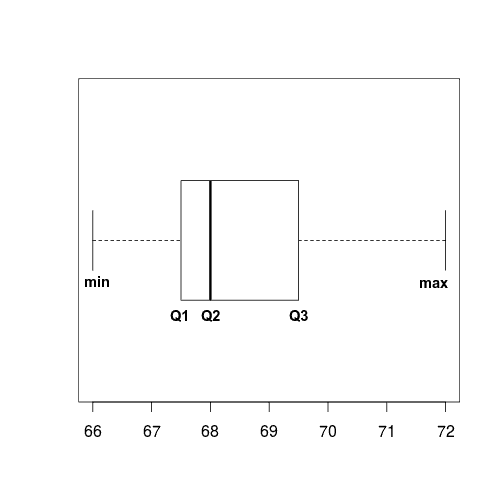
- \(Q_1 = 67.25\)
- \(Q_2 = 68\)
- \(Q_3 = 69.75\)
6.5.3 Interquartile Range (IQR)
- The Inter-Quartile Range is defined as the difference between the upper quartile and the lower quartile, that is, \[ \boxed{\text{Interquartile Range} = Q_3 - Q_1} \]
- IQR is a measure of variability in the central part (between \(Q_1\) and \(Q_3\)) of the data. The larger the IQR is, the more spread the central part of the data is.
- For the Height data, the IQR is \(69.75 - 67.25 = 2.5\)
6.5.4 Box Plot
- As always, we will be happy if we can see the data by a graph. For numerical data, except for stem-and-leaf plot and histogram, we can also make a box plot which shows \(5\) important values of the data.
- To draw a box plot,
- Draw the real number line horizontally;
- At each of minimum, lower quartile (\(Q_1\)), median (\(Q_2\)), upper quartile (\(Q_3\)) and maximum, draw a vertical line.
- Make a box between the lower quartile (\(Q_1\)) and the upper quartile (\(Q_3\)), with median (\(Q_2\)) inside it;
- the left part of the box is between the lower quartile (\(Q_1\)) and the median (\(Q_2\)),
- the right part of the box is between the median (\(Q_2\)) and the upper quartile (\(Q_3\)) and
- Make the left whisker between the minimum and the lower quartile (\(Q_1\))
- make the right whisker between the upper quartile (\(Q_3\)) and the maximum.
For the Height data, the box plot is
7 References
- Keller, Gerald. (2015). Statistics for Management and Economics, 10th Edition. Stamford: Cengage Learning.